# GRADED FUNCTION: linear_functiondeflinear_function():"""
Implements a linear function:
Initializes W to be a random tensor of shape (4,3)
Initializes X to be a random tensor of shape (3,1)
Initializes b to be a random tensor of shape (4,1)
Returns:
result -- runs the session for Y = WX + b
"""
np.random.seed(1)
### START CODE HERE ### (4 lines of code)
X = tf.constant(np.random.randn(3,1), name = "X")
W = tf.constant(np.random.randn(4,3), name = "X")
b = tf.constant(np.random.randn(4,1), name = "X")
Y = tf.add(tf.matmul(W,X),b)
### END CODE HERE ### # Create the session using tf.Session() and run it with sess.run(...) on the variable you want to calculate### START CODE HERE ###
sess = tf.Session()
result = sess.run(Y)
### END CODE HERE ### # close the session
sess.close()
return result
1.2 - Computing the sigmoid
# GRADED FUNCTION: sigmoiddefsigmoid(z):"""
Computes the sigmoid of z
Arguments:
z -- input value, scalar or vector
Returns:
results -- the sigmoid of z
"""### START CODE HERE ### ( approx. 4 lines of code)# Create a placeholder for x. Name it 'x'.
x = tf.placeholder(tf.float32, name = "X")
# compute sigmoid(x)
sigmoid = tf.sigmoid(x)
# Create a session, and run it. Please use the method 2 explained above. # You should use a feed_dict to pass z's value to x. with tf.Session() as sess:
# Run session and call the output "result"
result = sess.run(sigmoid, feed_dict = {x:z})
### END CODE HERE ###return result
1.3 - Computing the Cost
# GRADED FUNCTION: costdefcost(logits, labels):"""
Computes the cost using the sigmoid cross entropy
Arguments:
logits -- vector containing z, output of the last linear unit (before the final sigmoid activation)
labels -- vector of labels y (1 or 0)
Note: What we've been calling "z" and "y" in this class are respectively called "logits" and "labels"
in the TensorFlow documentation. So logits will feed into z, and labels into y.
Returns:
cost -- runs the session of the cost (formula (2))
"""### START CODE HERE ### # Create the placeholders for "logits" (z) and "labels" (y) (approx. 2 lines)
z = tf.placeholder(tf.float32, name = "z")
y = tf.placeholder(tf.float32, name = "y")
# Use the loss function (approx. 1 line)
cost = tf.nn.sigmoid_cross_entropy_with_logits(logits = z, labels = y)
# Create a session (approx. 1 line). See method 1 above.
sess = tf.Session()
# Run the session (approx. 1 line).
cost = sess.run(cost, feed_dict = {z:logits,y:labels})
# Close the session (approx. 1 line). See method 1 above.
sess.close()
### END CODE HERE ###return cost
1.4 - Using One Hot encodings
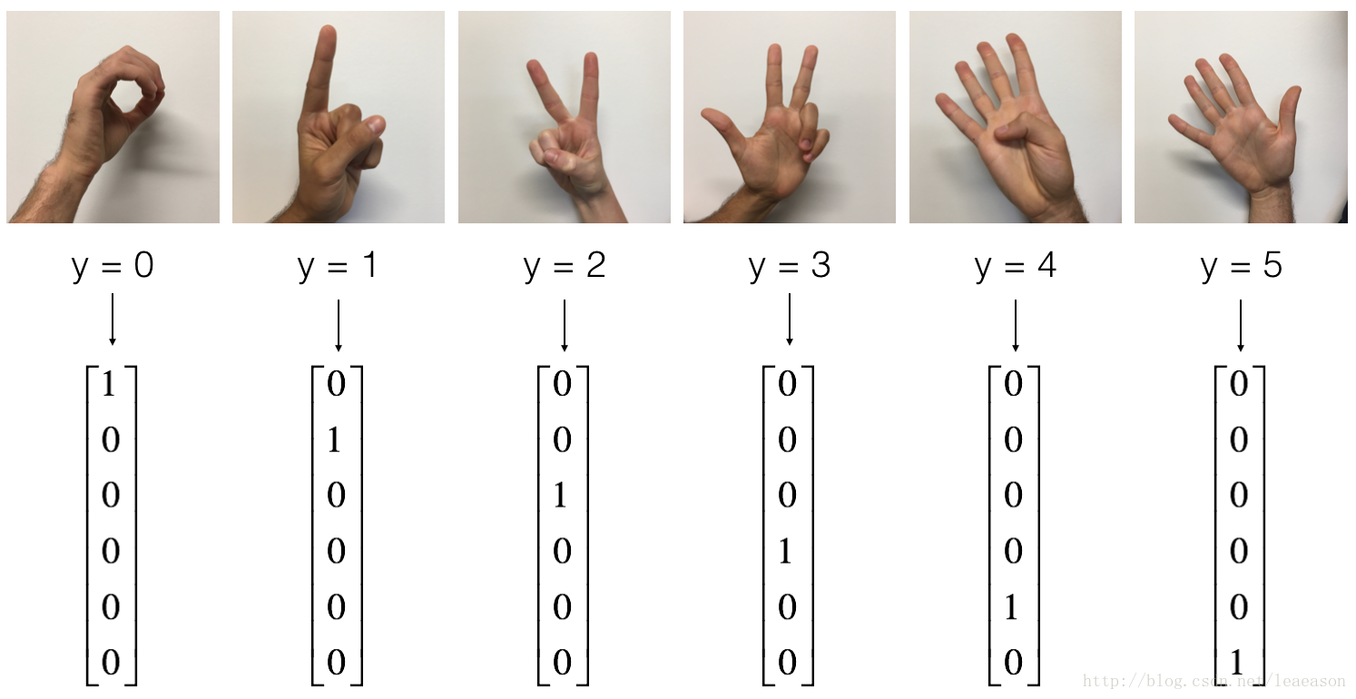
# GRADED FUNCTION: one_hot_matrixdefone_hot_matrix(labels, C):"""
Creates a matrix where the i-th row corresponds to the ith class number and the jth column
corresponds to the jth training example. So if example j had a label i. Then entry (i,j)
will be 1.
Arguments:
labels -- vector containing the labels
C -- number of classes, the depth of the one hot dimension
Returns:
one_hot -- one hot matrix
"""### START CODE HERE #### Create a tf.constant equal to C (depth), name it 'C'. (approx. 1 line)
C = tf.constant(C,name = "C")
# Use tf.one_hot, be careful with the axis (approx. 1 line)
one_hot_matrix = tf.one_hot(labels, C, axis=0)
# Create the session (approx. 1 line)
sess = tf.Session()
# Run the session (approx. 1 line)
one_hot = sess.run(one_hot_matrix)
# Close the session (approx. 1 line). See method 1 above.
sess.close()
### END CODE HERE ###return one_hot
1.5 - Initialize with zeros and ones
# GRADED FUNCTION: onesdefones(shape):"""
Creates an array of ones of dimension shape
Arguments:
shape -- shape of the array you want to create
Returns:
ones -- array containing only ones
"""### START CODE HERE #### Create "ones" tensor using tf.ones(...). (approx. 1 line)
ones = tf.ones(shape)
# Create the session (approx. 1 line)
sess = tf.Session()
# Run the session to compute 'ones' (approx. 1 line)
ones = sess.run(ones)
# Close the session (approx. 1 line). See method 1 above.
sess.close()
### END CODE HERE ###return ones
2 - Building your first neural network in tensorflow
2.0 - Problem statement: SIGNS Dataset
2.1 - Create placeholders
# GRADED FUNCTION: create_placeholdersdefcreate_placeholders(n_x, n_y):"""
Creates the placeholders for the tensorflow session.
Arguments:
n_x -- scalar, size of an image vector (num_px * num_px = 64 * 64 * 3 = 12288)
n_y -- scalar, number of classes (from 0 to 5, so -> 6)
Returns:
X -- placeholder for the data input, of shape [n_x, None] and dtype "float"
Y -- placeholder for the input labels, of shape [n_y, None] and dtype "float"
Tips:
- You will use None because it let's us be flexible on the number of examples you will for the placeholders.
In fact, the number of examples during test/train is different.
"""### START CODE HERE ### (approx. 2 lines)
X = tf.placeholder(tf.float32, shape =[n_x, None])
Y = tf.placeholder(tf.float32, shape =[n_y, None])
### END CODE HERE ### return X, Y
# GRADED FUNCTION: forward_propagationdefforward_propagation(X, parameters):"""
Implements the forward propagation for the model: LINEAR -> RELU -> LINEAR -> RELU -> LINEAR -> SOFTMAX
Arguments:
X -- input dataset placeholder, of shape (input size, number of examples)
parameters -- python dictionary containing your parameters "W1", "b1", "W2", "b2", "W3", "b3"
the shapes are given in initialize_parameters
Returns:
Z3 -- the output of the last LINEAR unit
"""# Retrieve the parameters from the dictionary "parameters"
W1 = parameters['W1']
b1 = parameters['b1']
W2 = parameters['W2']
b2 = parameters['b2']
W3 = parameters['W3']
b3 = parameters['b3']
### START CODE HERE ### (approx. 5 lines) # Numpy Equivalents:
Z1 = tf.add(tf.matmul(W1,X),b1) # Z1 = np.dot(W1, X) + b1
A1 = tf.nn.relu(Z1) # A1 = relu(Z1)
Z2 = tf.add(tf.matmul(W2,A1),b2) # Z2 = np.dot(W2, a1) + b2
A2 = tf.nn.relu(Z2) # A2 = relu(Z2)
Z3 = tf.add(tf.matmul(W3,Z2),b3) # Z3 = np.dot(W3,Z2) + b3### END CODE HERE ###return Z3
2.4 Compute cost
# GRADED FUNCTION: compute_cost defcompute_cost(Z3, Y):"""
Computes the cost
Arguments:
Z3 -- output of forward propagation (output of the last LINEAR unit), of shape (6, number of examples)
Y -- "true" labels vector placeholder, same shape as Z3
Returns:
cost - Tensor of the cost function
"""# to fit the tensorflow requirement for tf.nn.softmax_cross_entropy_with_logits(...,...)
logits = tf.transpose(Z3)
labels = tf.transpose(Y)
### START CODE HERE ### (1 line of code)
cost = tf.reduce_mean(tf.nn.softmax_cross_entropy_with_logits(logits = tf.transpose(Z3), labels =tf.transpose(Y) ))
### END CODE HERE ###return cost
2.5 - Backward propagation & parameter updates
2.6 - Building the model
defmodel(X_train, Y_train, X_test, Y_test, learning_rate = 0.0001,
num_epochs = 1500, minibatch_size = 32, print_cost = True):"""
Implements a three-layer tensorflow neural network: LINEAR->RELU->LINEAR->RELU->LINEAR->SOFTMAX.
Arguments:
X_train -- training set, of shape (input size = 12288, number of training examples = 1080)
Y_train -- test set, of shape (output size = 6, number of training examples = 1080)
X_test -- training set, of shape (input size = 12288, number of training examples = 120)
Y_test -- test set, of shape (output size = 6, number of test examples = 120)
learning_rate -- learning rate of the optimization
num_epochs -- number of epochs of the optimization loop
minibatch_size -- size of a minibatch
print_cost -- True to print the cost every 100 epochs
Returns:
parameters -- parameters learnt by the model. They can then be used to predict.
"""
ops.reset_default_graph() # to be able to rerun the model without overwriting tf variables
tf.set_random_seed(1) # to keep consistent results
seed = 3# to keep consistent results
(n_x, m) = X_train.shape # (n_x: input size, m : number of examples in the train set)
n_y = Y_train.shape[0] # n_y : output size
costs = [] # To keep track of the cost# Create Placeholders of shape (n_x, n_y)### START CODE HERE ### (1 line)
X, Y = create_placeholders(n_x, n_y)
### END CODE HERE #### Initialize parameters### START CODE HERE ### (1 line)
parameters = initialize_parameters()
### END CODE HERE #### Forward propagation: Build the forward propagation in the tensorflow graph### START CODE HERE ### (1 line)
Z3 = forward_propagation(X, parameters)
### END CODE HERE #### Cost function: Add cost function to tensorflow graph### START CODE HERE ### (1 line)
cost = compute_cost(Z3, Y)
### END CODE HERE #### Backpropagation: Define the tensorflow optimizer. Use an AdamOptimizer.### START CODE HERE ### (1 line)
optimizer = tf.train.AdamOptimizer(learning_rate = learning_rate).minimize(cost)
### END CODE HERE #### Initialize all the variables
init = tf.global_variables_initializer()
# Start the session to compute the tensorflow graphwith tf.Session() as sess:
# Run the initialization
sess.run(init)
# Do the training loopfor epoch in range(num_epochs):
epoch_cost = 0.# Defines a cost related to an epoch
num_minibatches = int(m / minibatch_size) # number of minibatches of size minibatch_size in the train set
seed = seed + 1
minibatches = random_mini_batches(X_train, Y_train, minibatch_size, seed)
for minibatch in minibatches:
# Select a minibatch
(minibatch_X, minibatch_Y) = minibatch
# IMPORTANT: The line that runs the graph on a minibatch.# Run the session to execute the "optimizer" and the "cost", the feedict should contain a minibatch for (X,Y).### START CODE HERE ### (1 line)
_ , minibatch_cost = sess.run([optimizer, cost], feed_dict={X: minibatch_X, Y: minibatch_Y})
### END CODE HERE ###
epoch_cost += minibatch_cost / num_minibatches
# Print the cost every epochif print_cost == Trueand epoch % 100 == 0:
print ("Cost after epoch %i: %f" % (epoch, epoch_cost))
if print_cost == Trueand epoch % 5 == 0:
costs.append(epoch_cost)
# plot the cost
plt.plot(np.squeeze(costs))
plt.ylabel('cost')
plt.xlabel('iterations (per tens)')
plt.title("Learning rate =" + str(learning_rate))
plt.show()
# lets save the parameters in a variable
parameters = sess.run(parameters)
print ("Parameters have been trained!")
# Calculate the correct predictions
correct_prediction = tf.equal(tf.argmax(Z3), tf.argmax(Y))
# Calculate accuracy on the test set
accuracy = tf.reduce_mean(tf.cast(correct_prediction, "float"))
print ("Train Accuracy:", accuracy.eval({X: X_train, Y: Y_train}))
print ("Test Accuracy:", accuracy.eval({X: X_test, Y: Y_test}))
return parameters
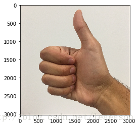
2.7 - Test with your own image (optional / ungraded exercise)
import scipy
from PIL import Image
from scipy import ndimage
## START CODE HERE ## (PUT YOUR IMAGE NAME)
my_image = "thumbs_up.jpg"## END CODE HERE ### We preprocess your image to fit your algorithm.
fname = "images/" + my_image
image = np.array(ndimage.imread(fname, flatten=False))
my_image = scipy.misc.imresize(image, size=(64,64)).reshape((1, 64*64*3)).T
my_image_prediction = predict(my_image, parameters)
plt.imshow(image)
print("Your algorithm predicts: y = " + str(np.squeeze(my_image_prediction)))