Initialization
import numpy as np
import matplotlib.pyplot as plt
import sklearn
import sklearn.datasets
from init_utils import sigmoid, relu, compute_loss, forward_propagation, backward_propagation
from init_utils import update_parameters, predict, load_dataset, plot_decision_boundary, predict_dec

%matplotlib inline
plt.rcParams['figure.figsize'] = (7.0, 4.0) # set default size of plots
plt.rcParams['image.interpolation'] = 'nearest'
plt.rcParams['image.cmap'] = 'gray'

# load image dataset: blue/red dots in circles
train_X, train_Y, test_X, test_Y = load_dataset()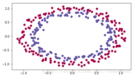
1 - Neural Network model
def model(X, Y, learning_rate = 0.01, num_iterations = 15000, print_cost = True, initialization = "he"):
"""
Implements a three-layer neural network: LINEAR->RELU->LINEAR->RELU->LINEAR->SIGMOID.
Arguments:
X -- input data, of shape (2, number of examples)
Y -- true "label" vector (containing 0 for red dots; 1 for blue dots), of shape (1, number of examples)
learning_rate -- learning rate for gradient descent
num_iterations -- number of iterations to run gradient descent
print_cost -- if True, print the cost every 1000 iterations
initialization -- flag to choose which initialization to use ("zeros","random" or "he")
Returns:
parameters -- parameters learnt by the model
"""
grads = {}
costs = [] # to keep track of the loss
m = X.shape[1] # number of examples
layers_dims = [X.shape[0], 10, 5, 1]
# Initialize parameters dictionary.
if initialization == "zeros":
parameters = initialize_parameters_zeros(layers_dims)
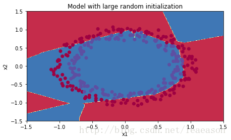
elif initialization == "random":
parameters = initialize_parameters_random(layers_dims)
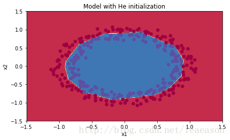
elif initialization == "he":
parameters = initialize_parameters_he(layers_dims)
# Loop (gradient descent)
for i in range(0, num_iterations):
# Forward propagation: LINEAR -> RELU -> LINEAR -> RELU -> LINEAR -> SIGMOID.
a3, cache = forward_propagation(X, parameters)
# Loss
cost = compute_loss(a3, Y)
# Backward propagation.
grads = backward_propagation(X, Y, cache)
# Update parameters.
parameters = update_parameters(parameters, grads, learning_rate)
# Print the loss every 1000 iterations
if print_cost and i % 1000 == 0:
print("Cost after iteration {}: {}".format(i, cost))
costs.append(cost)
# plot the loss
plt.plot(costs)
plt.ylabel('cost')
plt.xlabel('iterations (per hundreds)')
plt.title("Learning rate =" + str(learning_rate))
plt.show()
return parameters2 - Zero initialization
# GRADED FUNCTION: initialize_parameters_zeros

def initialize_parameters_zeros(layers_dims):
    """
    Arguments:
    layer_dims -- python array (list) containing the size of each layer.

    Returns:
    parameters -- python dictionary containing your parameters "W1", "b1", ..., "WL", "bL":
                    W1 -- weight matrix of shape (layers_dims[1], layers_dims[0])
                    b1 -- bias vector of shape (layers_dims[1], 1)
                    ...
                    WL -- weight matrix of shape (layers_dims[L], layers_dims[L-1])
                    bL -- bias vector of shape (layers_dims[L], 1)
    """

    parameters = {}
    L = len(layers_dims)            # number of layers in the network

    for l in range(1, L):
        ### START CODE HERE ### (≈ 2 lines of code)
        parameters['W' + str(l)] = np.zeros((layers_dims[l], layers_dims[l-1]))
        parameters['b' + str(l)] = np.zeros((layers_dims[l], 1))
        ### END CODE HERE ###
    return parameters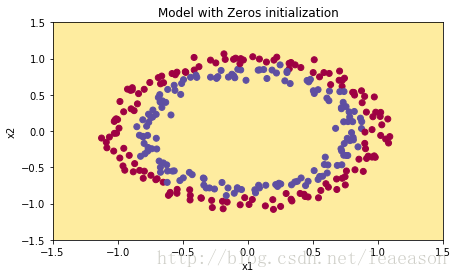
3 - Random initialization
def initialize_parameters_random(layers_dims):
    """
    Arguments:
    layer_dims -- python array (list) containing the size of each layer.

    Returns:
    parameters -- python dictionary containing your parameters "W1", "b1", ..., "WL", "bL":
                    W1 -- weight matrix of shape (layers_dims[1], layers_dims[0])
                    b1 -- bias vector of shape (layers_dims[1], 1)
                    ...
                    WL -- weight matrix of shape (layers_dims[L], layers_dims[L-1])
                    bL -- bias vector of shape (layers_dims[L], 1)
    """

    np.random.seed(3)               # This seed makes sure your "random" numbers will be the as ours
    parameters = {}
    L = len(layers_dims)            # integer representing the number of layers

    for l in range(1, L):
        ### START CODE HERE ### (≈ 2 lines of code)
        parameters['W' + str(l)] = np.random.randn(layers_dims[l], layers_dims[l-1])*10
        parameters['b' + str(l)] = np.zeros((layers_dims[l], 1))
        ### END CODE HERE ###

    return parameters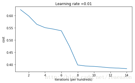
4 - He initialization
# GRADED FUNCTION: initialize_parameters_he

def initialize_parameters_he(layers_dims):
    """
    Arguments:
    layer_dims -- python array (list) containing the size of each layer.

    Returns:
    parameters -- python dictionary containing your parameters "W1", "b1", ..., "WL", "bL":
                    W1 -- weight matrix of shape (layers_dims[1], layers_dims[0])
                    b1 -- bias vector of shape (layers_dims[1], 1)
                    ...
                    WL -- weight matrix of shape (layers_dims[L], layers_dims[L-1])
                    bL -- bias vector of shape (layers_dims[L], 1)
    """

    np.random.seed(3)
    parameters = {}
    L = len(layers_dims) - 1 # integer representing the number of layers

    for l in range(1, L + 1):
        ### START CODE HERE ### (≈ 2 lines of code)
        parameters['W' + str(l)] = np.random.randn(layers_dims[l], layers_dims[l-1])*np.sqrt(2./layers_dims[l-1])
        parameters['b' + str(l)] = np.zeros((layers_dims[l], 1))
        ### END CODE HERE ###

    return parameters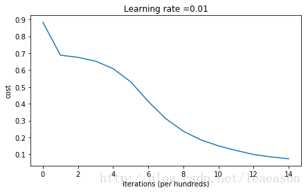
Regularization
1 - Non-regularized model
def model(X, Y, learning_rate = 0.3, num_iterations = 30000, print_cost = True, lambd = 0, keep_prob = 1):
"""
Implements a three-layer neural network: LINEAR->RELU->LINEAR->RELU->LINEAR->SIGMOID.
Arguments:
X -- input data, of shape (input size, number of examples)
Y -- true "label" vector (1 for blue dot / 0 for red dot), of shape (output size, number of examples)
learning_rate -- learning rate of the optimization
num_iterations -- number of iterations of the optimization loop
print_cost -- If True, print the cost every 10000 iterations
lambd -- regularization hyperparameter, scalar
keep_prob - probability of keeping a neuron active during drop-out, scalar.
Returns:
parameters -- parameters learned by the model. They can then be used to predict.
"""
grads = {}
costs = [] # to keep track of the cost
m = X.shape[1] # number of examples
layers_dims = [X.shape[0], 20, 3, 1]
# Initialize parameters dictionary.
parameters = initialize_parameters(layers_dims)
# Loop (gradient descent)
for i in range(0, num_iterations):
# Forward propagation: LINEAR -> RELU -> LINEAR -> RELU -> LINEAR -> SIGMOID.
if keep_prob == 1:
a3, cache = forward_propagation(X, parameters)
elif keep_prob < 1:
a3, cache = forward_propagation_with_dropout(X, parameters, keep_prob)
# Cost function
if lambd == 0:
cost = compute_cost(a3, Y)
else:
cost = compute_cost_with_regularization(a3, Y, parameters, lambd)
# Backward propagation.
assert(lambd==0 or keep_prob==1) # it is possible to use both L2 regularization and dropout,
# but this assignment will only explore one at a time
if lambd == 0 and keep_prob == 1:
grads = backward_propagation(X, Y, cache)
elif lambd != 0:
grads = backward_propagation_with_regularization(X, Y, cache, lambd)
elif keep_prob < 1:
grads = backward_propagation_with_dropout(X, Y, cache, keep_prob)
# Update parameters.
parameters = update_parameters(parameters, grads, learning_rate)
# Print the loss every 10000 iterations
if print_cost and i % 10000 == 0:
print("Cost after iteration {}: {}".format(i, cost))
if print_cost and i % 1000 == 0:
costs.append(cost)
# plot the cost
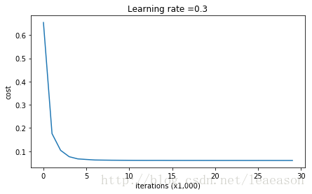
plt.plot(costs)
plt.ylabel('cost')
plt.xlabel('iterations (x1,000)')
plt.title("Learning rate =" + str(learning_rate))
plt.show()
return parameters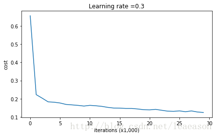

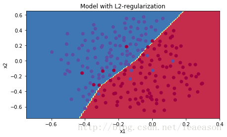
2 - L2 Regularization
# GRADED FUNCTION: compute_cost_with_regularization

def compute_cost_with_regularization(A3, Y, parameters, lambd):
    """
    Implement the cost function with L2 regularization. See formula (2) above.

    Arguments:
    A3 -- post-activation, output of forward propagation, of shape (output size, number of examples)
    Y -- "true" labels vector, of shape (output size, number of examples)
    parameters -- python dictionary containing parameters of the model

    Returns:
    cost - value of the regularized loss function (formula (2))
    """
    m = Y.shape[1]
    W1 = parameters["W1"]
    W2 = parameters["W2"]
    W3 = parameters["W3"]

    cross_entropy_cost = compute_cost(A3, Y) # This gives you the cross-entropy part of the cost

    ### START CODE HERE ### (approx. 1 line)
    L2_regularization_cost = (lambd/(2*m))*(np.sum(np.square(W1))+np.sum(np.square(W2))+np.sum(np.square(W3)))
    ### END CODER HERE ###

    cost = cross_entropy_cost + L2_regularization_cost

    return cost
# GRADED FUNCTION: backward_propagation_with_regularization
def backward_propagation_with_regularization(X, Y, cache, lambd):
"""
Implements the backward propagation of our baseline model to which we added an L2 regularization.
Arguments:
X -- input dataset, of shape (input size, number of examples)
Y -- "true" labels vector, of shape (output size, number of examples)
cache -- cache output from forward_propagation()
lambd -- regularization hyperparameter, scalar
Returns:
gradients -- A dictionary with the gradients with respect to each parameter, activation and pre-activation variables
"""
m = X.shape[1]
(Z1, A1, W1, b1, Z2, A2, W2, b2, Z3, A3, W3, b3) = cache
dZ3 = A3 - Y
### START CODE HERE ### (approx. 1 line)
dW3 = 1./m * np.dot(dZ3, A2.T) + (lambd/m)*W3
### END CODE HERE ###
db3 = 1./m * np.sum(dZ3, axis=1, keepdims = True)
dA2 = np.dot(W3.T, dZ3)
dZ2 = np.multiply(dA2, np.int64(A2 > 0))
### START CODE HERE ### (approx. 1 line)
dW2 = 1./m * np.dot(dZ2, A1.T) + (lambd/m)*W2
### END CODE HERE ###
db2 = 1./m * np.sum(dZ2, axis=1, keepdims = True)
dA1 = np.dot(W2.T, dZ2)
dZ1 = np.multiply(dA1, np.int64(A1 > 0))
### START CODE HERE ### (approx. 1 line)
dW1 = 1./m * np.dot(dZ1, X.T) + (lambd/m)*W1
### END CODE HERE ###
db1 = 1./m * np.sum(dZ1, axis=1, keepdims = True)
gradients = {"dZ3": dZ3, "dW3": dW3, "db3": db3,"dA2": dA2,
"dZ2": dZ2, "dW2": dW2, "db2": db2, "dA1": dA1,
"dZ1": dZ1, "dW1": dW1, "db1": db1}
return gradients
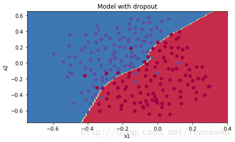
3 - Dropout
3.1 - Forward propagation with dropout
# GRADED FUNCTION: forward_propagation_with_dropout

def forward_propagation_with_dropout(X, parameters, keep_prob = 0.5):
    """
    Implements the forward propagation: LINEAR -> RELU + DROPOUT -> LINEAR -> RELU + DROPOUT -> LINEAR -> SIGMOID.

    Arguments:
    X -- input dataset, of shape (2, number of examples)
    parameters -- python dictionary containing your parameters "W1", "b1", "W2", "b2", "W3", "b3":
                    W1 -- weight matrix of shape (20, 2)
                    b1 -- bias vector of shape (20, 1)
                    W2 -- weight matrix of shape (3, 20)
                    b2 -- bias vector of shape (3, 1)
                    W3 -- weight matrix of shape (1, 3)
                    b3 -- bias vector of shape (1, 1)
    keep_prob - probability of keeping a neuron active during drop-out, scalar

    Returns:
    A3 -- last activation value, output of the forward propagation, of shape (1,1)
    cache -- tuple, information stored for computing the backward propagation
    """

    np.random.seed(1)

    # retrieve parameters
    W1 = parameters["W1"]
    b1 = parameters["b1"]
    W2 = parameters["W2"]
    b2 = parameters["b2"]
    W3 = parameters["W3"]
    b3 = parameters["b3"]

    # LINEAR -> RELU -> LINEAR -> RELU -> LINEAR -> SIGMOID
    Z1 = np.dot(W1, X) + b1
    A1 = relu(Z1)
    ### START CODE HERE ### (approx. 4 lines)         # Steps 1-4 below correspond to the Steps 1-4 described above.
    D1 = np.random.rand(A1.shape[0],A1.shape[1])                                         # Step 1: initialize matrix D1 = np.random.rand(..., ...)
    D1 =  D1<keep_prob                                        # Step 2: convert entries of D1 to 0 or 1 (using keep_prob as the threshold)
    A1 = A1*D1                                         # Step 3: shut down some neurons of A1
    A1 =  A1/keep_prob                                        # Step 4: scale the value of neurons that haven't been shut down
    ### END CODE HERE ###
    Z2 = np.dot(W2, A1) + b2
    A2 = relu(Z2)
    ### START CODE HERE ### (approx. 4 lines)
    D2 = np.random.rand(A2.shape[0],A2.shape[1])                                         # Step 1: initialize matrix D2 = np.random.rand(..., ...)
    D2 = D2<keep_prob                                         # Step 2: convert entries of D2 to 0 or 1 (using keep_prob as the threshold)
    A2 =  A2*D2                                        # Step 3: shut down some neurons of A2
    A2 = A2/keep_prob                                         # Step 4: scale the value of neurons that haven't been shut down
    ### END CODE HERE ###
    Z3 = np.dot(W3, A2) + b3
    A3 = sigmoid(Z3)

    cache = (Z1, D1, A1, W1, b1, Z2, D2, A2, W2, b2, Z3, A3, W3, b3)

    return A3, cache
3.2 - Backward propagation with dropout
# GRADED FUNCTION: backward_propagation_with_dropout

def backward_propagation_with_dropout(X, Y, cache, keep_prob):
    """
    Implements the backward propagation of our baseline model to which we added dropout.

    Arguments:
    X -- input dataset, of shape (2, number of examples)
    Y -- "true" labels vector, of shape (output size, number of examples)
    cache -- cache output from forward_propagation_with_dropout()
    keep_prob - probability of keeping a neuron active during drop-out, scalar

    Returns:
    gradients -- A dictionary with the gradients with respect to each parameter, activation and pre-activation variables
    """

    m = X.shape[1]
    (Z1, D1, A1, W1, b1, Z2, D2, A2, W2, b2, Z3, A3, W3, b3) = cache

    dZ3 = A3 - Y
    dW3 = 1./m * np.dot(dZ3, A2.T)
    db3 = 1./m * np.sum(dZ3, axis=1, keepdims = True)
    dA2 = np.dot(W3.T, dZ3)
    ### START CODE HERE ### (≈ 2 lines of code)
    dA2 = D2*dA2              # Step 1: Apply mask D2 to shut down the same neurons as during the forward propagation
    dA2 = dA2/keep_prob              # Step 2: Scale the value of neurons that haven't been shut down
    ### END CODE HERE ###
    dZ2 = np.multiply(dA2, np.int64(A2 > 0))
    dW2 = 1./m * np.dot(dZ2, A1.T)
    db2 = 1./m * np.sum(dZ2, axis=1, keepdims = True)

    dA1 = np.dot(W2.T, dZ2)
    ### START CODE HERE ### (≈ 2 lines of code)
    dA1 = D1*dA1              # Step 1: Apply mask D1 to shut down the same neurons as during the forward propagation
    dA1 = dA1/keep_prob              # Step 2: Scale the value of neurons that haven't been shut down
    ### END CODE HERE ###
    dZ1 = np.multiply(dA1, np.int64(A1 > 0))
    dW1 = 1./m * np.dot(dZ1, X.T)
    db1 = 1./m * np.sum(dZ1, axis=1, keepdims = True)

    gradients = {"dZ3": dZ3, "dW3": dW3, "db3": db3,"dA2": dA2,
                 "dZ2": dZ2, "dW2": dW2, "db2": db2, "dA1": dA1,
                 "dZ1": dZ1, "dW1": dW1, "db1": db1}

    return gradients