完整的视频课堂链接如下:
完整的视频课堂投影片连接:
前一課堂筆記連結:
Menu this round
- CPU vs GPU
- Deep Learning Frameworks
- Caffe / Caffe2
- Theano / TensorFlow
- Torch / PyTorch
CPU vs GPU
他们分别都是电脑的组成部分,CPU 安装在电路主板上,高性能的 CPU 还会连接散热铜管,并有很多针脚与“防呆”拼接设计,防止有人误装错方向;而 GPU 是像显卡一样装在电脑主板拓展槽里面的一个大型模块,因为其在运算的的时候需要大功率,所以一个 GPU 里面已经内置了风扇装置。(右边:GPU;左边:CPU)
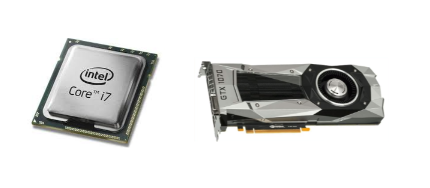
一台电脑中 CPU 基本上只能装一个,反之 GPU 则可以根据拓展槽的个数加装。
GPU stands for Graphics Processing Unit.
CPU stands for Computing Processing Unit.
他们两个有着个别的优势,CPU 善于处理多种复杂的运算,反观 GPU 更能够适应超级大规模的重复性平行运算,原本是多个算式的数学公式,我们可以藉由矩阵把他们圈成一个单元下的组成部分之一,这样一来,电脑就知道这个时候该开始平行运算,而这种特殊的情况一旦放到了 GPU 之中,其特点与长处就得以大放异采,这也是为什么我们之后建模的时候总是喜欢使用矩阵的模式去规范数据,而且用矩阵还要用 Numpy 这个 module 的矩阵,更进一步提升计算速度。
后面提到的 Framework 搭配上这些硬件,就可以更为有效率的分配硬件上的运算资源,让整体面临超级大量数据的时候运行速度得到好的优化。然而,如果不使用这些框架,也有以下的方式去部署 GPU 资源:CUDA(NVIDIA only);OpenCL(but usually slower)。但是这些部署方式都需要很仔细并小心的处理,才能够真正高效的把全部的硬件计算资源调用起来。
除了硬件的资源调用之外,data 在电脑里面的传输也是非常需要注意的事情,基于有 GPU 的情况下,算法的 model 是建立在 GPU 里面的,然而实际上的 data 是在硬盘里面存着的,快速喂食 GPU 数据的方法如下:
- 尽量使用 SSD 并舍弃传统的磁碟硬盘
- 可以事先预存 data 到缓存里面随时准备调用
- 事先让 CPU 预处理一些数据也能提升速度
Deep Learning Frameworks
市面上已经存在非常多种框架能够实践深度学习的功能,其中 caffe, pytorch, tensorflow 是最为常见的选择之一,当然不乏其他优秀的框架,但是这边主要集中描述此三类。
使用这些 Frameworks 的好处:
- 很容易的就可以创建计算流程图
- 很容易的计算流程图中每个节点的梯度值
- 很容易把这些计算流程套如 GPU 做运算速度的优化
import numpy as np
np.random.seed(0)

N, D = 3, 4
x = np.random.randn(N, D)
y = np.random.rnadn(N, D)
z = np.random.randn(N, D)

a = x * y
b = a + z
c = np.sum(b)

grad_c = 1.0
grad_b = grad_c * np.ones((N, D))
grad_a = grad)b.copy()
...
即便一个很简单的式子,在没有框架的辅助下,也会很常弄得自己焦头烂额,并且到最后还不能用 GPU 加速。因此框架的重要性显而易见了,使用 tensorflow 首先建立“node节点”,再安排节点该做的事,最后初始化所有的节点并使用 tf.Session() 运行所有过程,实际代码如下:
import numpy as np
np.random.seed(0)
import tensorflow as tf

N, D = 3, 4
# to construct the calculating graph to a specific location such as GPU,
# we can simply use this one line of code below.
with tf.device('/gpu:0'):
    x = tf.placeholder(tf.float32)
    y = tf.placeholder(tf.float32)
    z = tf.placeholder(tf.float32)
    # these are just spaces left for individual value to fill in later. it's empty now

    a = x * y
    b = a + z
    c = tf.reduce_sum(b)
    # these lines of code look are same as the previous example above

grad_x, grad_y, grad_z = tf.gradient(c, [x, y, z])
# we can simply get the value of gradient for individual variable by using this one line!

with tf.Session() as sess:
    values = {
        x: np.random.randn(N, D),
        y: np.random.randn(N, D),
        z: np.random.randn(N, D)
    }
    out = sess.run([c, grad_x, grad_y, grad_z], feed_dict=values)
    c_val, grad_x_val, grad_y_val, grad_z_val = out
而使用 pytorch 的话过程也是类似的,只是就这个例子而言会比 tensorflow 更为简单好懂,代码如下:
import torch
from torch.autograd import Variable

N, D = 3, 4
x = Variable(torch.randn(N, D).cuda(), requires_grad=True)
y = Variable(torch.randn(N, D).cuda(), requires_grad=True)
z = Variable(torch.randn(N, D).cuda(), requires_grad=True)
# .cuda() term is added for constructing on GPU just like how tf.device() has done.
# if there are no specific appointment, these structures will be built in CPU as default.

a = x * y
b = a + z
c = torch.sum(b)

c.backward()

print(x.grad.data)
print(y.grad.data)
print(z.grad.data)
Tensorflow: Neural Net
使用这个 framework 建立神经网络的步骤中,首先建立 computational graph ,再用 tf.Session() 函数去开启 .run 的功能,让 graph 被执行并达到训练的效果。
首先详述 computational graph 里面的结构,它是一个没有执行功能的流程图架构,由两个主要的元素组成:
- node 节点
这里是主要 variable 被赋值的地方,更准确的说应该是“赋值”这个动作发生的地方,至于是不是真的赋值成功了,那是另一回事,像 tf.placeholder(dtype, shape=None) 功能就是创一个空的节点(形象化比喻:占毛坑不拉屎)。 - edge 键
这里是主要用来规范每个节点之间的互动关系,他们该相加,相减,还是任何其他的操作,就像原子之间的键接,是把 nodes 之间编织成一个网络的主要手段。
一旦计算流程图绘制完毕后,接下来就是要把这些 node 做“初始化”,像是赋予他们生命力的一个过程,没有这个过程不但设置的很多参数都不能用之外,还会让程序报错。直到初始化这一步,tensorflow 都还没有开始任何的计算操作,都是在构建一个“图”而已,直到接下来用 tf.Session() 带出来的这段代码开始,才是实际要开始运算的起点。
在来解析 tf.Session() ,它是一个可以把这句话之前的所有代码打包封装成可以被整体执行的图的 function,在 .run( ) 里面的 object 会被直接运行,并且要是在得出 object 的计算结果之前需要预先计算的部分,也会一并涵盖入整体的计算范围,例如:c = a + 1; a = 4 + 3,计算 c 的时候需要先计算 a 的值,对于 tf 的 .run(c) 来说,a 的值也会跟着预处理,不用我们操心。
基本上大致的逻辑框架就是如此,下面是一个实际训练数据的代码范例:
import numpy as np
import tensorflow as tf

N, D, H = 64, 1000, 100
x = tf.placeholder(tf.float32, shape=(N, D))
y = tf.placeholder(tf.float32, shape=(N, D))
w1 = tf.Variable(tf.random_normal((D, H)))
w2 = tf.Variable(tf.random_normal((H, D)))
# till now, we can say that the nodes have all been created

h = tf.maximum(tf.matmul(x, w1), 0)
y_pred = tf.matmul(h, w2)
diff = y_pred - y
loss = tf.reduce_mean(tf.reduce_sum(diff*diff, axis=1))
# these lines are the edges to tell the operations between nodes

optimizer = tf.train.GradientDescentOptimizer(0.05)
updates = optimizer.minimize(loss)

with tf.Session() as sess:
    sess.run(tf.global_variables_initializer())
    value = {x: np.random.randn(N, D),
             y: np.random.randn(N, D)}
    losses = []
    for t in range(50):
        loss_val, _ = sess.run([loss, updates], feed_dict=value}
在 nodes 建立的过程中,有 placeholder and Variable 两种方式,后者是需要初始化的,但是前者由于特性是只占着毛坑,因此每一次 session 循环的时候都要重新 feed 进去一个值,这造成了前面提到由于数据提供速度不够快造成的瓶颈,nodes 搭建在 GPU 上反观 data 却是在硬盘里,因此当遇到多的数据点时,强烈建议使用 Variable 直接让 node 本身有值,可以很大省去数据传递的时间与低效。
...
x = tf.placeholder(tf.float32, shape=(N, D))
y = tf.placeholder(tf.float32, shape=(N, D))

init = tf.contrib.layers.xavier_initializer()
h = tf.layers.dense(inputs=x, units=H, activation=tf.nn.relu, kernel_initializer=init)
y_pred = tf.layers.dense(inputs=h, units=D, kernel_initializer=init)
# this is the way to build up the structure of neurons without explicitly written down the detail

loss = tf.losses.mean_squared_error(y_pred, y)
optimizer = tf.train.GradientDescentOptimizer(0.1)
updates = optimizer.minimize(loss)

with tf.Session() as sess:
    ...
一开始就提及到的流程图概念,原因就是 tensorflow 本身还提供了流程图“可视化”的功能,名为 tensorboard!可以在架构建立好之后,用图的形式把关系画成图
PyTorch: Three Levels of Abstraction
运行的原理大同小异,也是建立节点,设定节点之间的关系,最后执行。PyTorch 的向量几乎就像是 Numpy 的模式,只是它可以在 GPU 里面运行。
不过比较不好的是,他没有 graph,gradients 集成工具,或是 deep learning functions,凡是都是要自己来,他就真的像是 GPU 版本的 numpy一般,所有的梯度计算都要自己列算式:
import torch

dtype = torch.FloatTensor
# or use "torch.cuda.FloatTensor" to convert the model in to GPU
# to create random arrays for data and weights
N, D_in, H, D_out = 64, 1000, 100, 10
x = torch.randn(N, D_in).type(dtype)
y = torch.randn(N, D_out).type(dtype)
w1 = torch.randn(D_in, H).type(dtype)
w2 = torch.randn(H, D_out).type(dtype)

# the forward pass to list the functionality of a neural cell waiting for cycling
learning_rate = 1e-6
for t in range(500):
    h = x.mm(w1)
    h_relu = h.clamp(min=0)
    y_pred = h_relu.mm(w2)
    loss = (y_pred - y).pow(2).sum()

    # hand made backpropagation started from here
    grad_y_pred = 2.0 * (y_pred - y)
    grad_w2 = h_relu.t().mm(grad_y_pred)
    grad_h_relu = grad_y_pred.mm(w2.t())
    grad_h = grad_h_relu.clone()
    grad_h[h<0] = 0
    grad_w1 = x.t().mm(grad_h)

    w1 -= learning_rate * grad_w1
    w2 -= learning_rate * grad_w2
为了解决没有工具可用的问题,并且每次执行 for loop 都要重新一次架构图的描写,是一件很复杂且没效率的事情,因此我们必须自己创立这些缺失的 functions:
class ReLU(torch.autograd.Function):
    def forward(self, x):
        self.save_for_backward(x)
        return x.clamp(min=0)

    def backward(self, grad_y):
        x = self.saved_tensors
        grad_input = grad_y.clone()
        grad_input[x<0] = 0
        return grad_input
PyTorch 也有些 module:nn,optim,虽然没有像 tensorflow 那般强大,但是一般常用的功能如 MESLoss,Linear,也都包含在内了,下面是结合 class 与内置 module 的范例:
import torch
from torch.autograd import Variable

class TwoLayerNet(torch.nn.Module):
    def __init__(self, D_in, H, D_out):
        # to inherit TwoLayerNet class, use super()...
        super(TwoLayerNet, self).__init__()
        self.linear1 = torch.nn.Linear(D_in, H)
        self.linear2 = torch.nn.Linear(H, D_out)
    def forward(self, x):
        h_relu = self.linear1(x).clamp(min=0)
        y_pred = self.linear2(h_relu)
        return y_pred

N, D_in, H, D_out = 64, 1000, 100, 10
x = Variable(torch.randn(N, D_in))
y = Variable(torch.randn(N, D_out), requires_grad=False)
model = TwoLayerNet(D_in, H, D_out)

Criterion = torch.nn.MSELoss(size_average=False)
optimizer = torch.optim.SGD(model.parameters(), ir=1e-4)
for t in range(500):
    y_pred = model(x)
    loss = criterion(y_pred, y)

    optimizer.zero_grad()
    loss.backward()
    optimizer.step()
一旦重要的 codes 被打包成 function 之后,写起来就更为轻松了。
除了一些神经网络相关的 class 如 nn,optim 之外,还有一些数据处理与切分的 functions 可以非常方便达到我们预期结果,"DataLoader" 就是一例:
from torch.utils.data import TensorDataset, Dataloader
...
loader = DataLoader(TensorDataset(x, y), batch_size=8)
...
可以达到自动切分数据的效果,并且是在 torch 资料形态的状态完成的,方便许多。
Static vs Dynamic Graphs
前面两种最常见到在 python 上面使用的 neural network 工具:tensorflow vs pytorch,他们有个根本上的逻辑不同。
Statics:
先建立好图(里面包含了 nodes and edges)然后重复执行这个建立好的流程,数据喂入可以直接就先嵌在图里,或是等到了执行的时候再放进图中都可以,虽然这会牵涉到上面提及的:计算速度受限于资料传输数度影响,但可以因情况而自行选定解决方案。tensorflow 就是这种方法的代表。
好处是可以在建构好 graph 的时候,实际执行前能针对每一个流程做优化(optimize),并且一旦神经网络训练好了之后,由于整个 graph 是固定的,直接写在了 GPU 里面,运行的时候只需要 serialize 流程图,就可以不需要 code 去跑整个 model。
Dynamic:
先建立好节点 nodes,设定好参数,然后才在重复执行的步骤中告知这些 nodes 彼此之间运作关系,因此每次新的一轮回圈中,整张图就像被刷新了一样,是一个动态的过程,执行的代码而言也更接近整个神经网络原理的底层,没有太多的 package 或是 API 使用。pytorch 就是这个方法的代表。
好处是一旦遇到条件式,可以非常简单的使用 if... else... 解决问题,因为图每次都要重新刷新,可以让 condition 加入 loop 里面一起运行即可。并且如果遇到 Loops 的调整与深层定制,动态的逻辑就会非常占上风。其中 Recurrent Neural Network 就是他的一大应用。
Caffe
使用的语言是 C++ 而非 python,但是有 python 与 matlab 的关联,它也是一个高度集成的 Framework 不怎么需要自己设置代码,不过已经不怎么在学术上被使用。
建模的方式是在 prototxt file 中完成的,大部分只需要设定参数即可,但是一旦遇到大的神经网络,prototxt 文件就要编辑上千行的代码,是个很不好看的过程,有些人为了方便甚至使用 python 写好然后转译过去。
流程如下:
- Convert data like LMDB or h5py
- Define network with maybe countless lines of codes in prototxt file
- Define parameters and solvers, such as learning rate, stepsize, iteration... etc.
- Start training with corresponding commands:
./build/tools/caffe train \
    -gpu 0 \
    -model path/to/trainval.prototxt \
    -solver path/to/solver.prototxt \
    -weights path/to/pretrained_weights.caffemodel
改进之后的 Caffe2 也是基于 C++ 操作,他有更优化的 python interface,并且可以在 iOS 和 Android 上面跑。但 Caffe 不是这门课的主题 Framework,因此介绍较少。