文章目录
视频: 55、PyTorch的交叉熵、信息熵、二分类交叉熵、负对数似然、KL散度、余弦相似度的原理与代码讲解_哔哩哔哩_bilibili
这里是对该视频内容的较为完整的整理。
1.Corss Entropy Loss
PyTorch API:CrossEntropyLoss — PyTorch 1.13 documentation
1.1 介绍
参数:

- weight:指定权重,(dim),可选参数,可以给每个类指定一个权重。通常在训练数据中不同类别的样本数量差别较大时,可以使用权重来平衡。
- ignore_index:指定忽略一个真实值,(int),也就是手动忽略一个真实值。
- reduction:在[none, mean, sum]中选,string型。
none表示不降维,返回和target相同形状;mean表示对一个batch的损失求均值;sum表示对一个batch的损失求和。
输入:
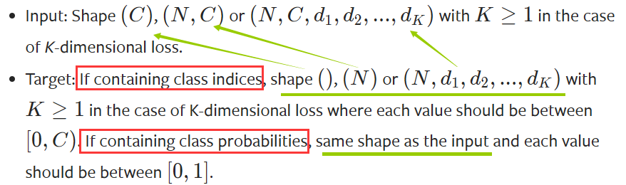
可以看到对于Target,是有两种情况的。如果Target是类别的索引,那么Target的shape是比Input的shape少了通道维;如果Target是类别的概率值,那么Target的shape是与Input的shape相同。具体可以看官网。
1.2 代码举例
import torch
import torch.nn as nn
import torch.nn.functional as F

# logits shape:[BS, NC]
batch_size = 2
num_class = 7

logits = torch.randn(batch_size, num_class)  # input unnormalized score
target_indices = torch.randint(num_class, size=(batch_size,))  # delta目标分布,是整形的索引 shape:(2,)
target_logits = torch.randn(batch_size, num_class)  # 非delta目标分布,概率分布 shape:[2,7]


ce_loss_fn = nn.CrossEntropyLoss()  # 实例化

## method 1 for CE loss
ce_loss = ce_loss_fn(logits, target_indices)
print(f"cross entropy loss1: {

      ce_loss}")

## method 2 for CE loss
ce_loss = ce_loss_fn(logits, torch.softmax(target_logits, dim=-1))
# 将target_logits 进行softmax在通道维上进行归一化成概率分布,和为1
print(f"cross entropy loss2: {

      ce_loss}")
输出结果均为标量:
cross entropy loss1: 3.269336700439453
cross entropy loss2: 2.0783615112304688
2.Negative Log Likelihood loss (NLL loss)
PyTorch API:NLLLoss — PyTorch 1.13 documentation
2.1 介绍
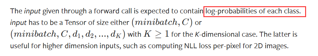
对于负对数似然Negative Log Likelihood loss(NLL loss)来说,input是每个类别的log-probabilities,而target只能为类别索引。实际上,能用cross entropy loss的地方就能用negative log-likelihood loss,这在后面的代码部分进行进一步验证。
2.2 代码举例
nll_fn = nn.NLLLoss()
nll_loss = nll_fn(torch.log(torch.softmax(logits, dim=-1)), target_indices)
print(f"negative log-likelihood loss: {

      nll_loss}")
沿用上面初始化的logits,对其在通道维上进行softmax得到归一化概率值,再取对数,从而获得batch_size个样本的每个class的log-probabilities。target_indices是类别索引。
输出结果为标量:
negative log-likelihood loss: 3.269336700439453
如果沿用上面CELoss的logits和target_indices的初始化值,可以看到cross entropy loss1和negative log-likelihood loss的输出结果是相同的。说明 c r o s s e n t r o p y l o s s = s o f t m a x + l o g + n l l l o s s cross \ entropy \ loss = softmax+log+nll\ loss cross entropy loss=softmax+log+nll loss (这是个人辅助记忆的方法,可能不太正规)。
3.Kullback-Leibler divergence loss (KL loss)
PyTorch API:KLDivLoss — PyTorch 1.13 documentation
3.1 介绍
P、Q相当于两个系统,KL距离的定义为:
D K L ( P ∣ ∣ Q ) = ∑ x ∈ X P ( x ) l o g ( P ( x ) Q ( x ) ) D_{KL}(P||Q)=\sum_{x\in \mathcal{X}}P(x)log \left ( \frac{P(x)}{Q(x)} \right ) DKL(P∣∣Q)=x∈X∑P(x)log(Q(x)P(x))
其中,P在前,即以P为基准,衡量Q相对于P来说的差距。如果P、Q两个系统分布相同,则 D K L ( P ∣ ∣ Q ) = 0 D_{KL}(P||Q)=0 DKL(P∣∣Q)=0。所以KL散度具有非负性。
对于官网上的公式来说,P等价于 y t r u e y_{true} ytrue,Q等价于 y p r e d y_{pred} ypred。
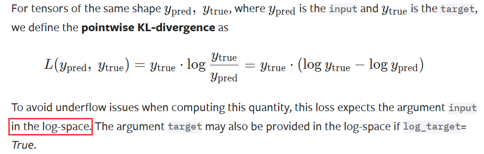
这里需要注意的是input和target的shape应该相同。而且,为了避免下溢的一些问题,期望 input是在log的空间传入进来的,而target可以是 log 空间,也可以是线性空间。
3.2 代码举例
kld_loss_fn = nn.KLDivLoss(reduction='mean')
kld_loss = kld_loss_fn(torch.log(torch.softmax(logits, dim=-1)), torch.softmax(target_logits, dim=-1))
print(f"Kullback-Leibler divergence loss : {

      kld_loss}")
输出结果为标量:
Kullback-Leibler divergence loss : 0.07705999910831451
4.验证 D K L ( P ∣ ∣ Q ) = H ( p , q ) − H ( p ) D_{KL}(P||Q)=H(p,q)-H(p) DKL(P∣∣Q)=H(p,q)−H(p)
4.1 介绍
首先从公式的角度来说明这个式子的正确性:

这个公式的意思是 p 、 q p、q p、q的KL散度 = p 、 q =p、q =p、q的交叉熵 − - − p p p 的信息熵。其中 p p p 的信息熵就是目标分布的信息熵。
4.2 代码验证
# 4.验证 CE = IE + KLD  交叉熵=信息熵+KL散度
# 交叉熵
ce_loss_fn_smaple = nn.CrossEntropyLoss(reduction="none")  # 能够输出每一个样本的loss,不进行平均
ce_loss_sample = ce_loss_fn_smaple(logits, torch.softmax(target_logits, dim=-1))  # (b,)
print(f"cross entropy loss sample: {

      ce_loss_sample}")

# KL散度
kld_loss_fn_sample = nn.KLDivLoss(reduction="none")
kld_loss_sample = kld_loss_fn_sample(torch.log(torch.softmax(logits, dim=-1)), torch.softmax(target_logits, dim=-1)).sum(-1)
print(f"Kullback-Leibler divergence loss sample: {

      kld_loss_sample}")

# 计算目标分布的信息熵
target_information_entropy = torch.distributions.Categorical(probs=torch.softmax(target_logits, dim=-1)).entropy()
print(f"information entropy sample: {

      target_information_entropy}")  # IE为常数,如果目标分布是delta分布,IE=0

# 验证 CE = IE + KLD 是否成立
print(torch.allclose(ce_loss_sample, kld_loss_sample + target_information_entropy))  # 比较两个浮点数
输出结果如下:
cross entropy loss sample: tensor([1.7736, 2.5585])
Kullback-Leibler divergence loss sample: tensor([0.1108, 1.1138])
information entropy sample: tensor([1.6628, 1.4447])
True
可以看到,最终的输出结果为True,说明公式成立。值得一提的是,由于在数据集中的target是确定的,所以其信息熵也是确定的,为常数。所以优化交叉熵损失和KL散度损失是等价的,只是在数值上相差一个常数。
5.Binary Cross Entropy loss (BCE loss)
PyTorch API:BCELoss — PyTorch 1.13 documentation
5.1 介绍
以上所介绍的都常使用于多分类问题,BCE loss二项交叉熵适用于二分类问题。API中的公式如下:
l n = − w n [ y n ⋅ log ( x n ) + ( 1 − y n ) ⋅ log ( 1 − x n ) ] l_n = - w_n[y_n \cdot \textup{\textrm{log}}(x_n)+(1-y_n) \cdot \textup{\textrm{log}}(1-x_n)] ln=−wn[yn⋅log(xn)+(1−yn)⋅log(1−xn)]
要求Target和Input是相同的维度,对于target,数值应该在0-1之间。
5.2 代码举例
# 5.调用Binary Cross Entropy loss (BCE loss) 二分类的损失函数

bce_loss_fn = nn.BCELoss()
logits = torch.randn(batch_size)
prob_1 = torch.sigmoid(logits)  # 使用sigmoid求出概率值
target = torch.randint(2, size=(batch_size,))  # 二分类,只有0和1
bce_loss = bce_loss_fn(prob_1, target.float())
print(f"binary Cross Entropy loss: {

      bce_loss}")


# 1) BCEWithLogitsLoss = sigmoid + BCELoss ,传入的未归一化的logits
bce_logits_loss_fn = nn.BCEWithLogitsLoss()
bce_logits_loss = bce_logits_loss_fn(logits, target.float())
print(f"binary Cross Entropy with logits loss: {

      bce_logits_loss}")
print(torch.allclose(bce_logits_loss, bce_loss))  # 比较两个浮点数


# 2) BCE Loss 是特殊的 NLL Loss
nll_fn = nn.NLLLoss()
prob_0 = 1 - prob_1.unsqueeze(-1)  # 在通道维升维 [BS, 1]
prob = torch.cat([prob_0, prob_1.unsqueeze(-1)], dim=-1)  # [BS, 2]
nll_loss_binary = nll_fn(torch.log(prob), target)
print(f"negative likelihood loss binary: {

      nll_loss_binary}")
print(torch.allclose(bce_loss, nll_loss_binary))  # 比较两个浮点数
输出结果如下:
binary Cross Entropy loss: 0.963399350643158
binary Cross Entropy with logits loss: 0.963399350643158
True
negative likelihood loss binary: 0.963399350643158
True
从输出结果中可以看出:1) B C E W i t h L o g i t s L o s s = s i g m o i d + B C E L o s s BCEWithLogitsLoss = sigmoid + BCELoss BCEWithLogitsLoss=sigmoid+BCELoss;2)BCE Loss 是特殊的 NLL Loss,NLL Loss可以处理多分类问题,当目标只有0、1两个索引时,也可以处理二分类的情况。
6.Cosine Similarity Loss
PyTorch API:CosineEmbeddingLoss — PyTorch 1.13 documentation
6.1 介绍
Cosine Embedding Loss基于余弦相似度,从而评估两个输入的量是相似的还是不相似的。在对比学习、自监督学习、学习图片或文本的相似度、搜索引擎图片搜索等中大量应用。
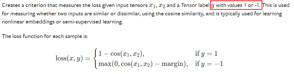
要求input1和input2的shape相同,target的值为1或者-1。
6.2 代码举例
cosine_loss_fn = nn.CosineEmbeddingLoss()
v1 = torch.randn(batch_size, 512)
v2 = torch.randn(batch_size, 512)
target = torch.randint(2, size=(batch_size, )) * 2 - 1  # 只能是-1~1
cosine_loss = cosine_loss_fn(v1, v2, target)
print(f"cosine similarity loss: {

      cosine_loss}")
输出结果为标量:
cosine similarity loss: 0.07631295919418335