Part 1: 词向量运算
欢迎来到本周第一个作业。
由于词嵌入的训练计算量庞大切耗费时间长,绝大部分机器学习人员都会导入一个预训练的词嵌入模型。
你将学到:
- 加载预训练单词向量,使用余弦测量相似度
- 使用词嵌入解决类别问题,比如 “Man is to Woman as King is to __”
- 修改文字嵌入以减少他们的性别偏见
导包
import numpy as np
from w2v_utils import *
w2v_utils 中有用的函数
from keras.models import Model
from keras.layers import Input, Dense, Reshape, merge
from keras.layers.embeddings import Embedding
from keras.preprocessing.sequence import skipgrams
from keras.preprocessing import sequence

import urllib.request
import collections
import os
import zipfile

import numpy as np
import tensorflow as tf

window_size = 3
vector_dim = 300
epochs = 1000

valid_size = 16     # Random set of words to evaluate similarity on.
valid_window = 100  # Only pick dev samples in the head of the distribution.
valid_examples = np.random.choice(valid_window, valid_size, replace=False)

def maybe_download(filename, url, expected_bytes):
    """Download a file if not present, and make sure it's the right size."""
    if not os.path.exists(filename):
        filename, _ = urllib.request.urlretrieve(url + filename, filename)
    statinfo = os.stat(filename)
    if statinfo.st_size == expected_bytes:
        print('Found and verified', filename)
    else:
        print(statinfo.st_size)
        raise Exception(
            'Failed to verify ' + filename + '. Can you get to it with a browser?')
    return filename


# Read the data into a list of strings.
def read_data(filename):
    """Extract the first file enclosed in a zip file as a list of words."""
    with zipfile.ZipFile(filename) as f:
        data = tf.compat.as_str(f.read(f.namelist()[0])).split()
    return data


def build_dataset(words, n_words):
    """Process raw inputs into a dataset."""
    count = [['UNK', -1]]
    count.extend(collections.Counter(words).most_common(n_words - 1))
    dictionary = dict()
    for word, _ in count:
        dictionary[word] = len(dictionary)
    data = list()
    unk_count = 0
    for word in words:
        if word in dictionary:
            index = dictionary[word]
        else:
            index = 0  # dictionary['UNK']
            unk_count += 1
        data.append(index)
    count[0][1] = unk_count
    reversed_dictionary = dict(zip(dictionary.values(), dictionary.keys()))
    return data, count, dictionary, reversed_dictionary

def collect_data(vocabulary_size=10000):
    url = 'http://mattmahoney.net/dc/'
    filename = maybe_download('text8.zip', url, 31344016)
    vocabulary = read_data(filename)
    print(vocabulary[:7])
    data, count, dictionary, reverse_dictionary = build_dataset(vocabulary,
                                                                vocabulary_size)
    del vocabulary  # Hint to reduce memory.
    return data, count, dictionary, reverse_dictionary

class SimilarityCallback:
    def run_sim(self):
        for i in range(valid_size):
            valid_word = reverse_dictionary[valid_examples[i]]
            top_k = 8  # number of nearest neighbors
            sim = self._get_sim(valid_examples[i])
            nearest = (-sim).argsort()[1:top_k + 1]
            log_str = 'Nearest to %s:' % valid_word
            for k in range(top_k):
                close_word = reverse_dictionary[nearest[k]]
                log_str = '%s %s,' % (log_str, close_word)
            print(log_str)

    @staticmethod
    def _get_sim(valid_word_idx):
        sim = np.zeros((vocab_size,))
        in_arr1 = np.zeros((1,))
        in_arr2 = np.zeros((1,))
        in_arr1[0,] = valid_word_idx
        for i in range(vocab_size):
            in_arr2[0,] = i
            out = validation_model.predict_on_batch([in_arr1, in_arr2])
            sim[i] = out
        return sim


def read_glove_vecs(glove_file):
    with open(glove_file, 'r') as f:
        words = set()
        word_to_vec_map = {}

        for line in f:
            line = line.strip().split()
            curr_word = line[0]
            words.add(curr_word)
            word_to_vec_map[curr_word] = np.array(line[1:], dtype=np.float64)

    return words, word_to_vec_map

def relu(x):
    """
    Compute the relu of x

    Arguments:
    x -- A scalar or numpy array of any size.

    Return:
    s -- relu(x)
    """
    s = np.maximum(0,x)

    return s


def initialize_parameters(vocab_size, n_h):
    """
    Arguments:
    layer_dims -- python array (list) containing the dimensions of each layer in our network

    Returns:
    parameters -- python dictionary containing your parameters "W1", "b1", "W2", "b2":
                    W1 -- weight matrix of shape (n_h, vocab_size)
                    b1 -- bias vector of shape (n_h, 1)
                    W2 -- weight matrix of shape (vocab_size, n_h)
                    b2 -- bias vector of shape (vocab_size, 1)
    """

    np.random.seed(3)
    parameters = {}

    parameters['W1'] = np.random.randn(n_h, vocab_size) / np.sqrt(vocab_size)
    parameters['b1'] = np.zeros((n_h, 1))
    parameters['W2'] = np.random.randn(vocab_size, n_h) / np.sqrt(n_h)
    parameters['b2'] = np.zeros((vocab_size, 1))

    return parameters

def softmax(x):
    """Compute softmax values for each sets of scores in x."""
    e_x = np.exp(x - np.max(x))
    return e_x / e_x.sum()
本作业中,我们使用50维的 Glove 向量来表示词。导入数据:
words, word_to_vec_map = read_glove_vecs('data/glove.6B.50d.txt')其中
- words: 词典中的词集合
- word_to_vec_map: 表示单词到向量映射的map。
one-hot向量不擅长表示向量相似度(内积为0), Glove 向量包含了单词更多的信息,下面看看如何使用 Glove 向量计算相似度。
1 余弦相似度
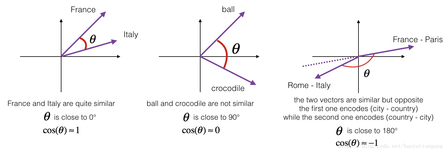
为了测量两个词的相似程度,需要测量两个词嵌入向量之间的相似程度。 给定两个向量u和v,余弦相似度定义如下:
分子表示两个向量的内积,分母是向量的模的乘积, 表示向量夹角,向量越近夹角越小,cos 值越大。
练习:实现cosine_similarity()方法来测量向量相似度
谨记:向量的模:向量每项平方加和再开方
# GRADED FUNCTION: cosine_similarity

def cosine_similarity(u, v):
    """
    Cosine similarity reflects the degree of similariy between u and v

    Arguments:
        u -- a word vector of shape (n,)
        v -- a word vector of shape (n,)

    Returns:
        cosine_similarity -- the cosine similarity between u and v defined by the formula above.
    """

    distance = 0.0

    ### START CODE HERE ###
    # Compute the dot product between u and v (≈1 line)
    dot = np.dot(u, v)
    # Compute the L2 norm of u (≈1 line)
    norm_u = np.sqrt(np.sum(u**2))

    # Compute the L2 norm of v (≈1 line)
    norm_v = np.sqrt(np.sum(v**2))
    # Compute the cosine similarity defined by formula (1) (≈1 line)
    cosine_similarity = dot / (norm_u * norm_v)
    ### END CODE HERE ###

    return cosine_similarity

#############################################

father = word_to_vec_map["father"]
mother = word_to_vec_map["mother"]
ball = word_to_vec_map["ball"]
crocodile = word_to_vec_map["crocodile"]
france = word_to_vec_map["france"]
italy = word_to_vec_map["italy"]
paris = word_to_vec_map["paris"]
rome = word_to_vec_map["rome"]

print("cosine_similarity(father, mother) = ", cosine_similarity(father, mother))
print("cosine_similarity(ball, crocodile) = ",cosine_similarity(ball, crocodile))
print("cosine_similarity(france - paris, rome - italy) = ",cosine_similarity(france - paris, rome - italy))

# cosine_similarity(father, mother) =  0.890903844289
# cosine_similarity(ball, crocodile) =  0.274392462614
# cosine_similarity(france - paris, rome - italy) =  -0.675147930817
期待的输出
| key | value |
|---|---|
| cosine_similarity(father, mother) | 0.890903844289 |
| cosine_similarity(ball, crocodile) | 0.274392462614 |
| cosine_similarity(france - paris, rome - italy) | -0.675147930817 |
2 单词类比推理
类比推理任务中需要实现”a is to b as c is to __” 比如”man is to woman as king is to queen”。我们需要找到单词 d,使得”e_b−e_a ≈ e_d−e_c”
也就是两组的差向量应该相似(仍然用 cos 来衡量)
练习:实现类比推理
# GRADED FUNCTION: complete_analogy

def complete_analogy(word_a, word_b, word_c, word_to_vec_map):
    """
    Performs the word analogy task as explained above: a is to b as c is to ____.

    Arguments:
    word_a -- a word, string
    word_b -- a word, string
    word_c -- a word, string
    word_to_vec_map -- dictionary that maps words to their corresponding vectors.

    Returns:
    best_word --  the word such that v_b - v_a is close to v_best_word - v_c, as measured by cosine similarity
    """

    # convert words to lower case
    word_a, word_b, word_c = word_a.lower(), word_b.lower(), word_c.lower()

    ### START CODE HERE ###
    # Get the word embeddings v_a, v_b and v_c (≈1-3 lines)
    e_a, e_b, e_c = word_to_vec_map[word_a], word_to_vec_map[word_b], word_to_vec_map[word_c]
    ### END CODE HERE ###

    words = word_to_vec_map.keys()
    max_cosine_sim = -100              # Initialize max_cosine_sim to a large negative number
    best_word = None                   # Initialize best_word with None, it will help keep track of the word to output

    # loop over the whole word vector set
    for w in words:
        # to avoid best_word being one of the input words, pass on them.
        if w in [word_a, word_b, word_c] :
            continue

        ### START CODE HERE ###
        # Compute cosine similarity between the vector (e_b - e_a) and the vector ((w's vector representation) - e_c)  (≈1 line)
        cosine_sim = cosine_similarity(e_b - e_a, word_to_vec_map[w] - e_c)

        # If the cosine_sim is more than the max_cosine_sim seen so far,
            # then: set the new max_cosine_sim to the current cosine_sim and the best_word to the current word (≈3 lines)
        if cosine_sim > max_cosine_sim:
            max_cosine_sim = cosine_sim
            best_word = w
        ### END CODE HERE ###

    return best_word

####################################################

triads_to_try = [('italy', 'italian', 'spain'), ('india', 'delhi', 'japan'), ('man', 'woman', 'boy'), ('small', 'smaller', 'large')]
for triad in triads_to_try:
    print ('{} -> {} :: {} -> {}'.format( *triad, complete_analogy(*triad,word_to_vec_map)))

# italy -> italian :: spain -> spanish
# india -> delhi :: japan -> tokyo
# man -> woman :: boy -> girl
# small -> smaller :: large -> larger
期待的输出
| key | value |
|---|---|
| italy -> italian | spain -> spanish |
| india -> delhi | japan -> tokyo |
| man -> woman | boy -> girl |
| small -> smaller | large -> larger |
你可以自己试试:small->smaller as big->?
谨记
- cos 是衡量向量相似度的好方法
- 对于 NLP 应用,使用一个预训练的模型开始工作是一个不错的选择
3 消除词向量偏见 (可选)
在下面的练习中,你将检查词嵌入中的性别偏见,并研究减少偏见的算法。 这部分涉及到一些线性代数,不要害怕,都是比较简单的。
先看看与性别有关的 Glove 词嵌入。 那么 g 向量认为就是性别有关的向量。
g = word_to_vec_map['woman'] - word_to_vec_map['man']
print(g)

# [-0.087144    0.2182     -0.40986    -0.03922    -0.1032      0.94165
#  -0.06042     0.32988     0.46144    -0.35962     0.31102    -0.86824
#   0.96006     0.01073     0.24337     0.08193    -1.02722    -0.21122
#   0.695044   -0.00222     0.29106     0.5053     -0.099454    0.40445
#   0.30181     0.1355     -0.0606     -0.07131    -0.19245    -0.06115
#  -0.3204      0.07165    -0.13337    -0.25068714 -0.14293    -0.224957
#  -0.149       0.048882    0.12191    -0.27362    -0.165476   -0.20426
#   0.54376    -0.271425   -0.10245    -0.32108     0.2516     -0.33455
#  -0.04371     0.01258   ]
然后利用 cos 计算不同单词的差向量与 g 向量的相似度,考虑什么是正相关什么是负相关。
print ('List of names and their similarities with constructed vector:')

# girls and boys name
name_list = ['john', 'marie', 'sophie', 'ronaldo', 'priya', 'rahul', 'danielle', 'reza', 'katy', 'yasmin']

for w in name_list:
    print (w, cosine_similarity(word_to_vec_map[w], g))

# List of names and their similarities with constructed vector:
# john -0.23163356146
# marie 0.315597935396
# sophie 0.318687898594
# ronaldo -0.312447968503
# priya 0.17632041839
# rahul -0.169154710392
# danielle 0.243932992163
# reza -0.079304296722
# katy 0.283106865957
# yasmin 0.233138577679
注意到女性名称与 g 正相关多一些,男性名字与 g负相关多一些。
再试试其他的词
print('Other words and their similarities:')
word_list = ['lipstick', 'guns', 'science', 'arts', 'literature', 'warrior','doctor', 'tree', 'receptionist',
             'technology',  'fashion', 'teacher', 'engineer', 'pilot', 'computer', 'singer']
for w in word_list:
    print (w, cosine_similarity(word_to_vec_map[w], g))

# Other words and their similarities:
# lipstick 0.276919162564
# guns -0.18884855679
# science -0.0608290654093
# arts 0.00818931238588
# literature 0.0647250443346
# warrior -0.209201646411
# doctor 0.118952894109
# tree -0.0708939917548
# receptionist 0.330779417506
# technology -0.131937324476
# fashion 0.0356389462577
# teacher 0.179209234318
# engineer -0.0803928049452
# pilot 0.00107644989919
# computer -0.103303588739
# singer 0.185005181365
令人惊讶的是这些与本应中立的词也有的不同的性别偏见,例如,“电脑”更接近“男人”,而“文学”更接近“女人”。
下面使用Boliukbasi等人2016年的算法来减少向量的偏见。应该保留性别相关的单词(actor/actress或grandmother/grandfather),中和那些与性别无关的单词(receptionist/technology)。
我们将采用不同的方式来处理这两种不同类型的词对。
3.1 中和无关性别的单词偏见
对于一个无关性别的单词,应该将其性别偏见消除,也就是将词向量分解为 g 方向和 g⊥方向,我们消除 g 方向的分量,仅保持g⊥方向的分量即可。
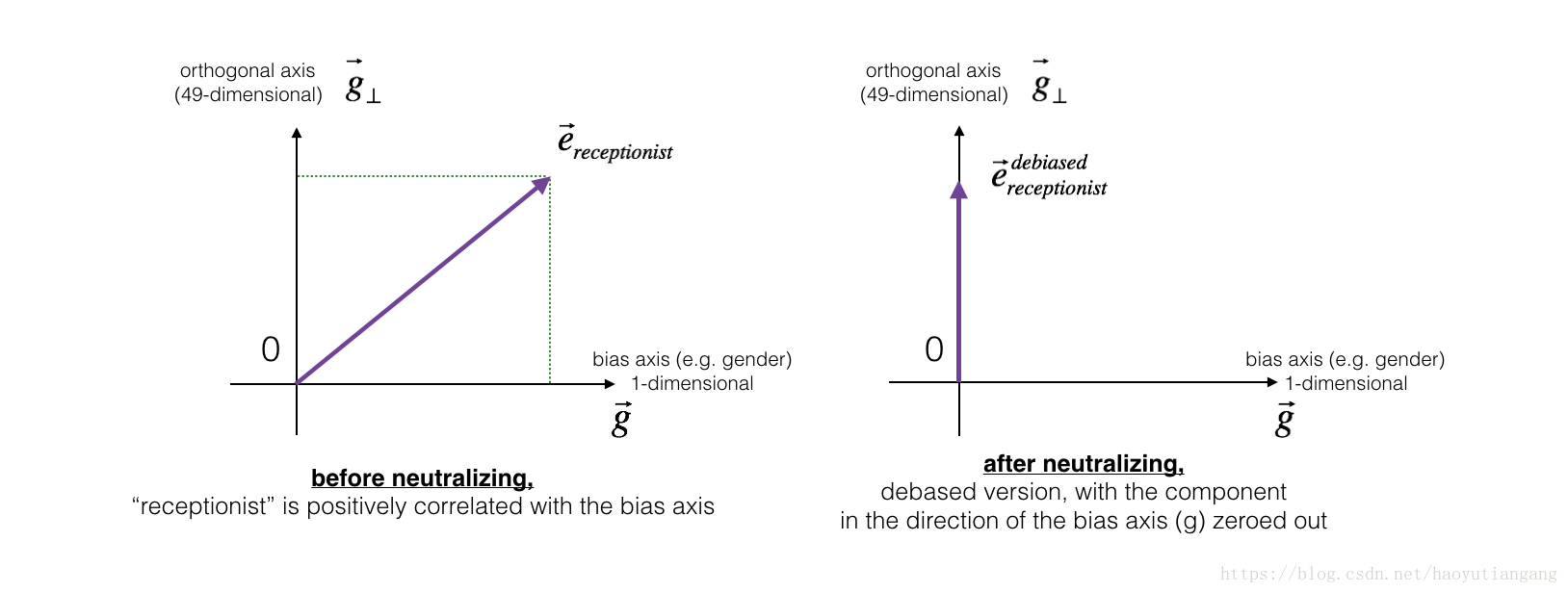
练习:实现 neutralize() 函数消除性别无关单词的性别偏见
给定一个词嵌入向量 e, 如下计算消除偏见后的向量。
- 先计算 e 向量在 g 方向上的分量
- 再用 e 减去上述分量即为无偏方向上的分量
def neutralize(word, g, word_to_vec_map):
    """
    Removes the bias of "word" by projecting it on the space orthogonal to the bias axis.
    This function ensures that gender neutral words are zero in the gender subspace.

    Arguments:
        word -- string indicating the word to debias
        g -- numpy-array of shape (50,), corresponding to the bias axis (such as gender)
        word_to_vec_map -- dictionary mapping words to their corresponding vectors.

    Returns:
        e_debiased -- neutralized word vector representation of the input "word"
    """

    ### START CODE HERE ###
    # Select word vector representation of "word". Use word_to_vec_map. (≈ 1 line)
    e = word_to_vec_map[word]

    # Compute e_biascomponent using the formula give above. (≈ 1 line)
    e_biascomponent = np.dot(e, g) / np.square(np.linalg.norm(g)) * g

    # Neutralize e by substracting e_biascomponent from it
    # e_debiased should be equal to its orthogonal projection. (≈ 1 line)
    e_debiased = e - e_biascomponent
    ### END CODE HERE ###

    return e_debiased

######################################################

e = "receptionist"
print("cosine similarity between " + e + " and g, before neutralizing: ", cosine_similarity(word_to_vec_map["receptionist"], g))

e_debiased = neutralize("receptionist", g, word_to_vec_map)
print("cosine similarity between " + e + " and g, after neutralizing: ", cosine_similarity(e_debiased, g))

# cosine similarity between receptionist and g, before neutralizing:  0.330779417506
# cosine similarity between receptionist and g, after neutralizing:  -3.26732746085e-17
期待的输出:
| key | value |
|---|---|
| cosine similarity between receptionist and g, before neutralizing: | 0.330779417506 |
| cosine similarity between receptionist and g, after neutralizing: | -3.26732746085e-17 |
第二个值非常小,近似为0
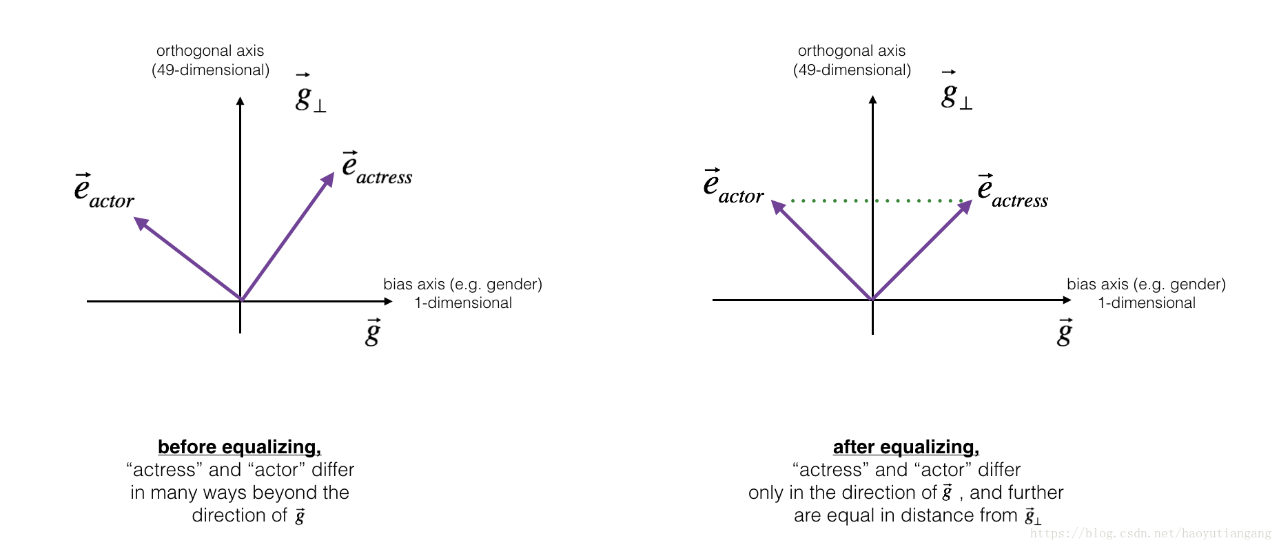
3.2 性别相关词汇的均衡算法
接下来,我们看看消除偏见如何应用于性别单词对:比如 actress/actor。
- 首先,希望将性别单词对向量设置为仅性别不同,所以应该在g⊥分量上相等。
- 其次,为了保证与中和过的无关向量距离相等,需要设置为在g分量上基于对称轴g⊥对称。
代码
def equalize(pair, bias_axis, word_to_vec_map):
    """
    Debias gender specific words by following the equalize method described in the figure above.

    Arguments:
    pair -- pair of strings of gender specific words to debias, e.g. ("actress", "actor")
    bias_axis -- numpy-array of shape (50,), vector corresponding to the bias axis, e.g. gender
    word_to_vec_map -- dictionary mapping words to their corresponding vectors

    Returns
    e_1 -- word vector corresponding to the first word
    e_2 -- word vector corresponding to the second word
    """

    ### START CODE HERE ###
    # Step 1: Select word vector representation of "word". Use word_to_vec_map. (≈ 2 lines)
    w1, w2 = pair
    e_w1, e_w2 = word_to_vec_map[w1], word_to_vec_map[w2]

    # Step 2: Compute the mean of e_w1 and e_w2 (≈ 1 line)
    mu = (e_w1 + e_w2) / 2

    # Step 3: Compute the projections of mu over the bias axis and the orthogonal axis (≈ 2 lines)
    mu_B = np.dot(mu, bias_axis) / np.sum(bias_axis**2) * bias_axis
    mu_orth = mu - mu_B

    # Step 4: Use equations (7) and (8) to compute e_w1B and e_w2B (≈2 lines)
    e_w1B = np.dot(e_w1, bias_axis) / np.sum(bias_axis**2) * bias_axis
    e_w2B = np.dot(e_w2, bias_axis) / np.sum(bias_axis**2) * bias_axis

    # Step 5: Adjust the Bias part of e_w1B and e_w2B using the formulas (9) and (10) given above (≈2 lines)
    corrected_e_w1B = np.sqrt(np.abs(1-np.sum(mu_orth**2))) * (e_w1B - mu_B)/np.linalg.norm(e_w1-mu_orth-mu_B)
    corrected_e_w2B =np.sqrt(np.abs(1-np.sum(mu_orth**2))) * (e_w2B - mu_B)/np.linalg.norm(e_w2-mu_orth-mu_B)

    # Step 6: Debias by equalizing e1 and e2 to the sum of their corrected projections (≈2 lines)
    e1 = corrected_e_w1B + mu_orth
    e2 = corrected_e_w2B + mu_orth

    ### END CODE HERE ###

    return e1, e2

######################################################

print("cosine similarities before equalizing:")
print("cosine_similarity(word_to_vec_map[\"man\"], gender) = ", cosine_similarity(word_to_vec_map["man"], g))
print("cosine_similarity(word_to_vec_map[\"woman\"], gender) = ", cosine_similarity(word_to_vec_map["woman"], g))
print()
e1, e2 = equalize(("man", "woman"), g, word_to_vec_map)
print("cosine similarities after equalizing:")
print("cosine_similarity(e1, gender) = ", cosine_similarity(e1, g))
print("cosine_similarity(e2, gender) = ", cosine_similarity(e2, g))

# cosine similarities before equalizing:
# cosine_similarity(word_to_vec_map["man"], gender) =  -0.117110957653
# cosine_similarity(word_to_vec_map["woman"], gender) =  0.356666188463
#
# cosine similarities after equalizing:
# cosine_similarity(e1, gender) =  -0.700436428931
# cosine_similarity(e2, gender) =  0.700436428931
期待的输出
均衡化之前的 cos相似度
| key | value |
|---|---|
| cosine_similarity(word_to_vec_map[“man”], gender) | -0.117110957653 |
| cosine_similarity(word_to_vec_map[“woman”], gender) | 0.356666188463 |
均衡化之后的 cos相似度
| key | value |
|---|---|
| cosine_similarity(u1, gender) | -0.700436428931 |
| cosine_similarity(u2, gender) | 0.700436428931 |
这里 g 向量仅用了
, 如果用多个性别对的平均值则效果更好,你可以尝试一下
恭喜!你已经完成本作业。
引用
- 偏见消除算法:Bolukbasi et al., 2016, Man is to Computer Programmer as Woman is to
Homemaker? Debiasing Word Embeddings - GloVe 词嵌入:Jeffrey Pennington, Richard Socher, and Christopher D. Manning. (https://nlp.stanford.edu/projects/glove/)