https://blog.csdn.net/To_be_to_thought/article/details/81780397阐释Batch Gradient Descent、Stochastic Gradient Descent、MiniBatch Gradient Descent具体原理。
对于梯度下降算法,当参数特别多时容易发现,速度会变慢,需要迭代的次数更多。优化速度与学习率、梯度变化量息息相关,如何自适应地在优化过程中调整学习率和梯度变化有利于加快梯度下降的求解过程,比如在陡峭的地方变化的梯度大一点,学习率大一点等等。
下面三种算法都是基于指数加权移动平均法考虑前面梯度对当前梯度的影响来对梯度、学习率作调整,从而更快收敛。
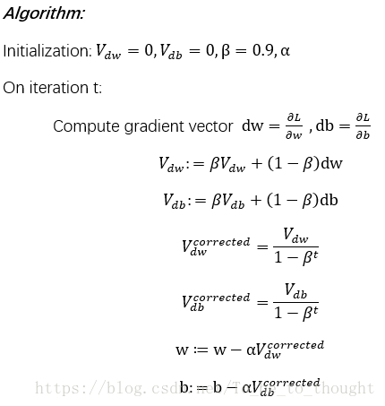
动量梯度下降算法(Momentum):
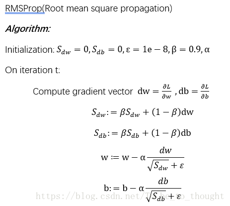
前向均方根梯度下降算法 RMSProp(Root mean square propagation):
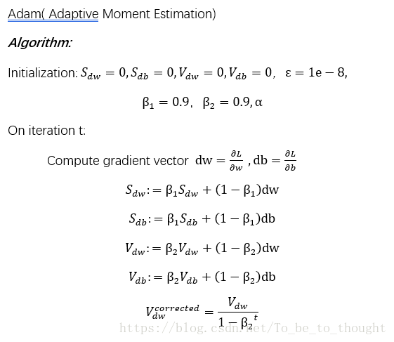
自适应估计算法(Adam)
以上算法流程均参考吴恩达老师《改善深层神经网络》视频内容,谢谢老师的仔细讲解!
下面算法实现和测试:
import numpy as np
import math
import matplotlib.pyplot as plt

#批量梯度下降法求最小值解 所有矩阵运算一律将ndarray转为matrix,以矩阵形式存储的向量一律转为列形式(n行一列的矩阵)
#alpha为学习速率,eps为一个特别小接近于0的值,循环种终止条件:1.达到最大迭代次数   2.损失函数变化量小于eps
#x_matrix为样本集数据,y_list为真实值标签
def Gradient_Descent(x_matrix,y_list,alpha,max_iter,eps):
    m,n=np.shape(x_matrix)
    #x_matrix=normalize(x_matrix)
    y_matrix=np.matrix(y_list).T
    new_X=np.matrix(np.ones((m,n+1)))
    theta=np.matrix(np.random.rand(n+1)).T#随机生成待求参数列向量,theta行数等于new_X的列数
    for i in range(m):
        new_X[i,1:n+1]=x_matrix[i,0:n]
    last_cost=0   #上一次损失函数值,初值为0
    index=0
    loss_record=[]
    cost=cost_function(new_X,y_matrix,theta)
    while abs(last_cost-cost)>eps and index<=max_iter:
        last_cost=cost
        theta[0]=theta[0]-alpha*1/m*sum(new_X*theta-y_matrix)
        theta[1:n+1]=theta[1:n+1]-alpha*1/m*sum(new_X.T*(new_X*theta-y_matrix))
        cost=cost_function(new_X,y_matrix,theta)
        index+=1
        loss_record.append(cost)
        print(str(index)+" "+str(abs(last_cost-cost)))
    return theta,loss_record

#动量梯度下降
#alpha为学习率 beta为加权系数 max_iter为最大迭代次数 eps1为损失函数变化量阈值 eps2为梯度变化的阈值
def GD_Momentum(X,y,alpha,beta,max_iter,eps1,eps2):
    m,n_features = X.shape
    new_X = np.column_stack((X,np.ones(m)))
    theta = np.random.random(n_features+1)
    init = np.zeros(n_features+1) #指数加权移动平均法的v初值
    itera = 0
    loss_record = []
    last_cost = 0 #上一轮计算的theta对应的损失函数值
    cost = cost_function(new_X,y,theta) #当前参数向量theta下的损失函数值
    loss_record.append(cost)
    while itera < max_iter and abs(cost-last_cost) > eps1:
        last_cost = cost
        gradient = np.dot(new_X.T,(np.dot(new_X,theta)-y))
        v=beta * init[:] + (1-beta) * gradient
        theta[:] = theta[:]-alpha*1/m*v
        init[:] = v[:]
        cost = cost_function(new_X,y,theta)
        print("loss function:"+str(cost))
        itera += 1
        loss_record.append(cost)
    return theta,loss_record

#Root Mean Square Propagation的梯度下降法
#alpha为全局学习率 beta为衰减速率 max_iter为最大迭代次数 eps1为损失函数变化量阈值 eps2为微小扰动1e-8
def GD_RMSprop(X,y,alpha,beta,max_iter,eps1,eps):
    m,n_features = X.shape     #m为样本数,n_features为特征数
    new_X = np.column_stack((X,np.ones(m)))
    theta = np.random.random(n_features+1)
    init_S = np.zeros(n_features+1)   #指数加权移动平均法的v初值
    itera = 0
    loss_record = []
    last_cost = 0 #上一轮计算的theta对应的损失函数值
    cost = cost_function(new_X,y,theta) #当前参数向量theta下的损失函数值
    loss_record.append(cost)
    while itera<max_iter and abs(cost-last_cost)>eps1:
        last_cost = cost
        gradient = np.dot(new_X.T,(np.dot(new_X,theta)-y))
        mean_square = beta * init_S[:] + (1-beta) * np.square(gradient)
        theta[:] = theta[:]-alpha * 1/m * gradient/(np.sqrt(mean_square)+eps)
        init_S[:] = mean_square[:]
        cost=cost_function(new_X,y,theta)
        print("loss function:"+str(cost))
        itera += 1
        loss_record.append(cost)
    return theta,loss_record

# Adaptive Moment Estimation的梯度下降法
# alpha为全局学习率 beta1为v的衰减速率向量,一般取0.9  beta2为S的衰减速率向量,一般取0.9 max_iter为最大迭代次数 eps1为损失函数变化量阈值 eps2为微小扰动1e-8
# v和S初值为0
def GD_Adam(X,y,alpha,beta1,beta2,max_iter,eps1,eps2):
    m,n_features = X.shape               #m为样本数,n_features为特征数
    new_X = np.column_stack((X,np.ones(m)))
    theta = np.random.random(n_features+1)
    init_v = np.zeros(n_features+1)      #指数加权移动平均法的初值
    init_S = np.zeros(n_features+1)
    itera = 0
    loss_record = []
    last_cost = 0 #上一轮计算的theta对应的损失函数值
    cost = cost_function(new_X,y,theta) #当前参数向量theta下的损失函数值
    loss_record.append(cost)
    while itera < max_iter and abs(cost-last_cost) > eps1:
        last_cost = cost
        gradient = np.dot(new_X.T,(np.dot(new_X,theta)-y))
        v = beta1 * init_v[:] + (1-beta1) * gradient
        S = beta2 * init_S[:] + (1-beta2) * np.square(gradient)
        v_corrected = v / (1 - np.power(beta1,itera+1)) #偏差矫正
        S_corrected = S / (1 - np.power(beta2,itera+1))
        theta[:] = theta[:] - alpha * 1/m * v_corrected / (np.sqrt(S_corrected) + eps2)
        init_v[:] = v_corrected[:]
        init_S[:] = S_corrected[:]
        cost = cost_function(new_X,y,theta)
        print("loss function:"+str(cost))
        itera += 1
        loss_record.append(cost)
    return theta,loss_record
测试代码:
X,y_list = file2matrix('H:/Machine Learning in Action/Ch08/ex0.txt')
y = np.reshape(y_list,len(y_list))
theta4,record4=GD_Momentum(X,y,0.01,0.9,1000,1e-10,1e-9)
theta5,record5 = GD_RMSprop(X,y,0.1,0.9,100000,1e-10,1e-8)
theta6,record6 = GD_Adam(X,y,0.1,0.9,0.9,500000,1e-10,1e-8)
plt.plot(np.arange(1,len(record5)+1),record5)
参数求解结果都比较接近,损失函数衰减图这里就不展示了!