参考 ： https://www.scratchapixel.com/lessons/mathematics-physics-for-computer-graphics/monte-carlo-methods-mathematical-foundations

Probability Density Function (PDF)

When a function such as the normal distribution defines a continuous probability distribution (such as the way height is distributed

among an adult popupulation), this function is called a probabilify density function (or pdf). In other words, pdfs are used for

continuous random variables and pmfs are used for discrete random variables. In computer graphics, we almost always deal with

pdfs. In short:

• the probability mass function (pmf) is the probability distribution of discrete random variable,
• the probability distribution function (pdf) is the probability distribution of a continuous random variable.

The PDF can be used to calculate the probability that a random variable lies within an interval:

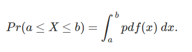
From this expression, it is clear that a PDF must always integrate to one over the full extent of its domain.

（PDF 其实就是 连续随机变量的 概率分布函数）

Cumulative Distribution Function (CDF)

Computing the CDF itself is a simple as adding the contribution of the current sample to the sum of all previous samples that

were already computed.

however of course, the more samples you use, the closer you get to its actual "true" shape. This is illustrated in the following

figure in which you can see the CDF of the function approximated with 10 samples (red) and 30 samples (green) compared to

the actual CDF (in blue). As you can see the more samples, the closer we get to the actual CDF.

Example：

What are CDFs useful for? In probability theory the are useful for computing things such as "what is the probability of getting

any of the first N possible outcomes of a random variable X". Let's take an example. We know that a dice has 6 possible

outcomes, it could either be 1, 2, 3, 4, 5 or 6. And we also know that each of these outcomes has probability 1/6. Now, if we

want to know the probability of getting any number lower or equal to 4 when we throw this dice, what we need to do, is sum up

the probability of having a 1, a 2, a 3 and a 4. We can write this mathematically as:

We have summed up the probabilities of the first N given possible outcomes (where N in this example is equal 4). If we plot the

result of this summation for Pr(X <=1), Pr(X <= 2), ... up to Pr(X <= 6), we get the diagram in figure 4, which as you can guess,

is the CDF (in green) of the probability function (in red) of our random variable. It is easier to explain the use of CDFs using a

discrete random variable (our dice example), however keep in mind that the idea applies to both discrete and continuous

probability functions.

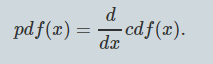
Note that CDFs are (always) monotonically(单调) increasing functions (which means that the PDF is always non-negative). It's not strictly monotic though. There may be intervals of constancy. Also from a mathematical point of view, a PDF can be seen as the derivative(导数) of its CDF: