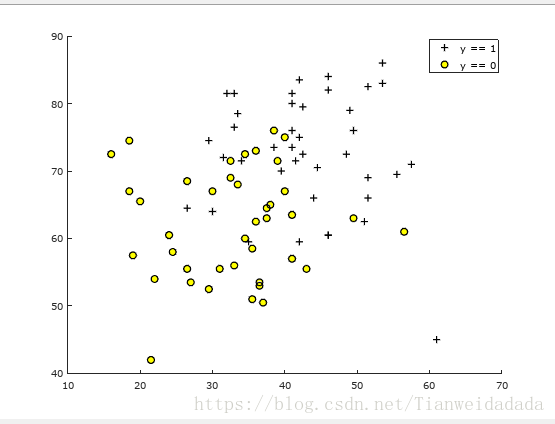
仍然使用之前的根据学生两学期分数,预测录取情况
主程序:
X = load('ex4x.dat');
y = load('ex4y.dat');
plotData(X,y);
[m,n] = size(X);
X = [ones(m,1),X];
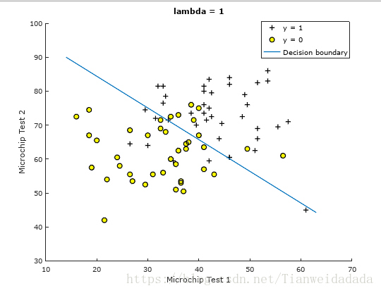
lambda = 1;
%[cost,grad] = costFunction(theta,X,y,lambda);
%fprintf('Cost at initial theta (zeros): %f\n', cost);
init_theta = zeros(n+1,1);
options = optimset('GradObj', 'on', 'MaxIter', 400);
f = @(t)(costFunction(t, X, y, lambda));
[theta, J, exit_flag] = fminunc(f, init_theta, options);
% Plot Boundary
plotDecisionBoundary(theta, X, y);
hold on;
title(sprintf('lambda = %g', lambda))
% Labels and Legend
xlabel('Microchip Test 1')
ylabel('Microchip Test 2')
legend('y = 1', 'y = 0', 'Decision boundary')
hold off;
% Compute accuracy on our training set
p = predict(theta, X);
fprintf('Train Accuracy: %f\n', mean(double(p == y)) * 100);
画原始的两学期分数分布图:
function plotData(X, y)
    figure;
    hold on;
    pos = find(y == 1);
    neg = find(y == 0);
    plot(X(pos, 1), X(pos, 2), 'k+', 'LineWidth', 2, 'MarkerSize', 7);
    plot(X(neg, 1), X(neg, 2), 'ko', 'MarkerFaceColor', 'y', 'MarkerSize', 7);
    legend('y == 1','y == 0');
    hold off;
end
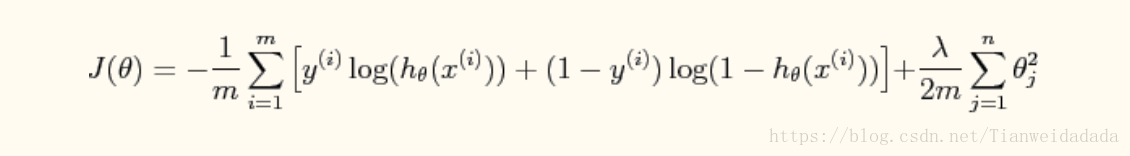
代价函数:
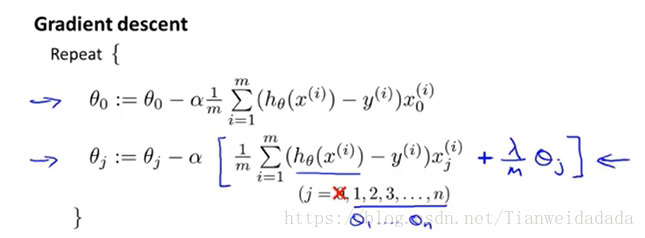
梯度(正则化,theta0不参与正则化):
function [J, grad] = costFunction(theta,X,y,lambda)
  m = length(y);
  %grad = zeros(m,1);
  sig = inline('1./(1+exp(-z))');
  grad = zeros(size(theta));
  J = 1/m*(sum(-y.*log(sig(X*theta))-(1-y).*log(1-sig(X*theta)))) +lambda/(2*m)*sum(theta(2:size(theta)).^2);%计算代价
  for j = 1:size(theta)
    if j == 1
      grad(j) = 1/m*sum((sig(X*theta)-y)'*X(:,j));
    else
      grad(j) = 1/m*sum((sig(X*theta)-y)'*X(:,j)) + lambda/m*theta(j);
    end
  end
end
画图里面包含了各种情况(这里只是用了最简单的那种):
function plotDecisionBoundary(theta, X, y)
%PLOTDECISIONBOUNDARY Plots the data points X and y into a new figure with
%the decision boundary defined by theta
%   PLOTDECISIONBOUNDARY(theta, X,y) plots the data points with + for the
%   positive examples and o for the negative examples. X is assumed to be
%   a either
%   1) Mx3 matrix, where the first column is an all-ones column for the
%      intercept.
%   2) MxN, N>3 matrix, where the first column is all-ones

    % Plot Data
    plotData(X(:,2:3), y);
    hold on

    if size(X, 2) <= 3
        % Only need 2 points to define a line, so choose two endpoints
        plot_x = [min(X(:,2))-2,  max(X(:,2))+2];

        % Calculate the decision boundary line
        plot_y = (-1./theta(3)).*(theta(2).*plot_x + theta(1));

        % Plot, and adjust axes for better viewing
        plot(plot_x, plot_y)

        % Legend, specific for the exercise
        legend('Admitted', 'Not admitted', 'Decision Boundary')
        axis([10, 70, 30, 100])
    else
        % Here is the grid range
        u = linspace(-1, 1.5, 50);
        v = linspace(-1, 1.5, 50);

        z = zeros(length(u), length(v));
        % Evaluate z = theta*x over the grid
        for i = 1:length(u)
            for j = 1:length(v)
                z(i,j) = mapFeature(u(i), v(j))*theta;
            end
        end
        z = z'; % important to transpose z before calling contour

        % Plot z = 0
        % Notice you need to specify the range [0, 0]
        contour(u, v, z, [0, 0], 'LineWidth', 2)
    end
    hold off

end
预测:
function p = predict(theta, X)
    sig = inline('1./(1+exp(-z))');
    p = sig(X * theta) >= 0.5;
end
参考博客:点击打开链接
数据源:点击打开链接