建模与调参
学习目标
掌握机器学习模型的建模与调参过程
内容介绍
-
线性回归模型:
-
线性回归对于特征的要求;
-
处理长尾分布;
-
理解线性回归模型;
-
-
模型性能验证:
-
评价函数与目标函数;
-
交叉验证方法;
-
留一验证方法;
-
针对时间序列问题的验证;
-
绘制学习率曲线;
-
绘制验证曲线;
-
-
嵌入式特征选择:
-
Lasso回归;
-
Ridge回归;
-
决策树;
-
-
模型对比:
-
常用线性模型;
-
常用非线性模型;
-
-
模型调参:
-
贪心调参方法;
-
网格调参方法;
-
贝叶斯调参方法;
-
代码示例
import pandas as pd

import numpy as np

import warnings

warnings.filterwarnings('ignore')
#定义reduce_men_usage函数,通过调整数据类型帮助我们减少数据所占内存空间

def reduce_mem_usage(df):

    start_men = df.memory_usage().sum()

    print('memory usage of dataframe is {:.2f} MB'.format(start_men))

    for col in df.columns:

        col_type = df[col].dtype

        if col_type != object:

            c_min = df[col].min()

            c_max = df[col].max()

            if str(col_type)[:3] == 'int':

                if c_min > np.iinfo(np.int8).min and c_max < np.iinfo(np.int8).max:

                    df[col] = df[col].astype(np.int8)

                elif c_min > np.iinfo(np.int16).min and c_max < np.iinfo(np.int16).max:

                    df[col] = df[col].astype(np.int16)

                elif c_min > np.iinfo(np.int32).min and c_max < np.iinfo(np.int32).max:

                    df[col] = df[col].astype(np.int32)

                elif c_min > np.iinfo(np.int64).min and c_max < np.iinfo(np.int64).max:

                    df[col] = df[col].astype(np.int64)

            else:

                if c_min > np.finfo(np.float16).min and c_max < np.finfo(np.float16).max:

                    df[col] = df[col].astype(np.float16)

                elif c_min > np.finfo(np.float32).min and c_max < np.finfo(np.float32).max:

                    df[col] = df[col].astype(np.float32)

                else:

                    df[col] = df[col].astype(np.float64)

        else:

            df[col] = df[col].astype('category')

    end_men = df.memory_usage().sum()

    print('Memory usage after optimization is :{:.2f} MB'.format(end_men))

    print('Decreased by {:.1f}%'.format(100*(start_men - end_men)/start_men))

    return df


sample_feature = reduce_mem_usage(pd.read_csv('data_for_tree.csv'))

#sample_feature.head()
memory usage of dataframe is 62099624.00 MB

Memory usage after optimization is :16520255.00 MB

Decreased by 73.4%
continuous_feature_names = [x for x in sample_feature.columns if x not in ['price','brand','model','brand']]

print(continuous_feature_names)

sample_feature = sample_feature.dropna().replace('-', 0).reset_index(drop=True)

sample_feature['notRepairedDamage'] = sample_feature['notRepairedDamage'].astype(np.float32)

train = sample_feature[continuous_feature_names + ['price']]

train_x = train[continuous_feature_names]

train_y = train['price']
['SaleID', 'name', 'bodyType', 'fuelType', 'gearbox', 'power', 'kilometer', 'notRepairedDamage', 'seller', 'offerType', 'v_0', 'v_1', 'v_2', 'v_3', 'v_4', 'v_5', 'v_6', 'v_7', 'v_8', 'v_9', 'v_10', 'v_11', 'v_12', 'v_13', 'v_14', 'train', 'used_time', 'city', 'brand_amount', 'brand_price_average', 'brand_price_max', 'brand_price_median', 'brand_price_min', 'brand_price_std', 'brand_price_sum', 'power_bin']
#train_x.head()
train_y.head()
0    1850.0

1    6222.0

2    5200.0

3    8000.0

4    3500.0

Name: price, dtype: float64
#1、简单建模,训练线性回归模型,查看截距与权重

from sklearn.linear_model import LinearRegression

model = LinearRegression(normalize=True)

model = model.fit(train_x, train_y)

sorted(dict(zip(continuous_feature_names, model.coef_)).items(), key=lambda x:x[1], reverse=True)
[('v_6', 3367064.341641952),

 ('v_8', 700675.5609398864),

 ('v_9', 170630.27723221222),

 ('v_7', 32322.661932025392),

 ('v_12', 20473.670796989394),

 ('v_3', 17868.07954151005),

 ('v_11', 11474.938996718518),

 ('v_13', 11261.764560017724),

 ('v_10', 2683.920090609242),

 ('gearbox', 881.8225039249613),

 ('fuelType', 363.90425072161565),

 ('bodyType', 189.60271012074494),

 ('city', 44.9497512052328),

 ('power', 28.55390161675131),

 ('brand_price_median', 0.5103728134078974),

 ('brand_price_std', 0.45036347092632434),

 ('brand_amount', 0.1488112039506708),

 ('brand_price_max', 0.0031910186703149753),

 ('SaleID', 5.3559899198567324e-05),

 ('seller', 2.4531036615371704e-06),

 ('train', 4.246830940246582e-07),

 ('offerType', -7.235445082187653e-06),

 ('brand_price_sum', -2.175006868187898e-05),

 ('name', -0.00029800127130847845),

 ('used_time', -0.0025158943328449923),

 ('brand_price_average', -0.40490484510113794),

 ('brand_price_min', -2.246775348688707),

 ('power_bin', -34.42064411726649),

 ('v_14', -274.7841180776088),

 ('kilometer', -372.897526660709),

 ('notRepairedDamage', -495.19038446298714),

 ('v_0', -2045.0549573540754),

 ('v_5', -11022.986240523212),

 ('v_4', -15121.731109858125),

 ('v_2', -26098.29992055678),

 ('v_1', -45556.189297264835)]
from matplotlib import pyplot as plt

subsample_index = np.random.randint(low=0, high=len(train_y),size=50)#随机抽取50个点验证

plt.scatter(train_x['v_9'][subsample_index], train_y[subsample_index], color='black')

plt.scatter(train_x['v_9'][subsample_index], model.predict(train_x.loc[subsample_index]), color='blue')

plt.xlabel('v_9')

plt.ylabel('price')

plt.legend(['True Price','Predicted Price'],loc='upper right')

print('The predicted price is obvious different from true price')

plt.show()
The predicted price is obvious different from true price
<Figure size 640x480 with 1 Axes>
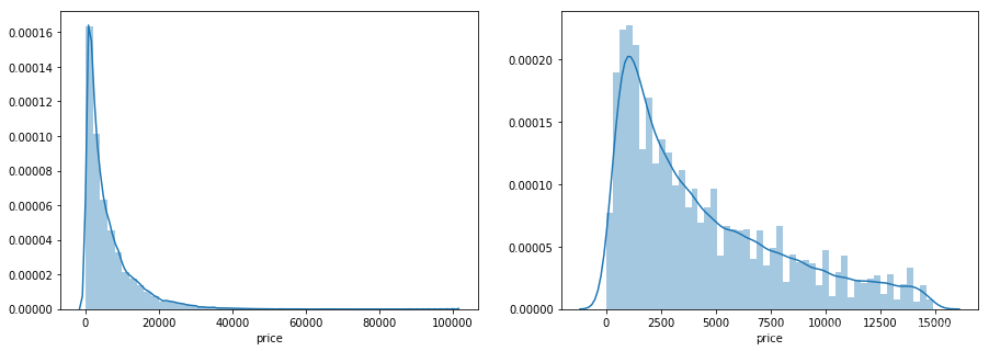
import seaborn as sns

print('It is clear to see the price shows a typical exponential distribution')

plt.figure(figsize=(15,5))

plt.subplot(1,2,1)

sns.distplot(train_y)

plt.subplot(1,2,2)

sns.distplot(train_y[train_y < train_y.quantile(0.9)]) #将长尾截断
It is clear to see the price shows a typical exponential distribution


<matplotlib.axes._subplots.AxesSubplot at 0x17cbe231c18>
![[外链图片转存失败,源站可能有防盗链机制,建议将图片保存下来直接上传(img-qR3hcGGy-1585460408912)(output_7_3.png)]](https://img-blog.csdnimg.cn/20200329134844225.png?x-oss-process=image/watermark,type_ZmFuZ3poZW5naGVpdGk,shadow_10,text_aHR0cHM6Ly9ibG9nLmNzZG4ubmV0L3dlaXhpbl80Mzk1OTI0OA==,size_16,color_FFFFFF,t_70)
#对标签进行log(x+1)变换使其贴近于正态分布,加一是为了防止底数为0

train_y_ln = np.log(train_y+1)

import seaborn as sns

print('The transformed price seems like normal distribution')

plt.figure(figsize=(15,5))

plt.subplot(1,2,1)

sns.distplot(train_y_ln)

plt.subplot(1,2,2)

sns.distplot(train_y_ln[train_y_ln < train_y.quantile(0.9)])
The transformed price seems like normal distribution
<matplotlib.axes._subplots.AxesSubplot at 0x17cbe53ffd0>
![[外链图片转存失败,源站可能有防盗链机制,建议将图片保存下来直接上传(img-4cBRUryw-1585460408915)(output_8_3.png)]](https://img-blog.csdnimg.cn/20200329134930218.png?x-oss-process=image/watermark,type_ZmFuZ3poZW5naGVpdGk,shadow_10,text_aHR0cHM6Ly9ibG9nLmNzZG4ubmV0L3dlaXhpbl80Mzk1OTI0OA==,size_16,color_FFFFFF,t_70)
model = model.fit(train_x, train_y_ln)

print('intercept:'+str(model.intercept_))

sorted(dict(zip(continuous_feature_names, model.coef_)).items(), key=lambda x:x[1], reverse=True)
intercept:18.75074946557562

[('v_9', 8.052409900567515),

 ('v_5', 5.7642365966517515),

 ('v_12', 1.6182081236790782),

 ('v_1', 1.479831058296809),

 ('v_11', 1.1669016563609707),

 ('v_13', 0.9404711296034489),

 ('v_7', 0.713727308356328),

 ('v_3', 0.6837875771083226),

 ('v_0', 0.008500518010020237),

 ('power_bin', 0.00849796930289155),

 ('gearbox', 0.00792237727832305),

 ('fuelType', 0.006684769706828705),

 ('bodyType', 0.004523520092702963),

 ('power', 0.0007161894205359341),

 ('brand_price_min', 3.334351114747353e-05),

 ('brand_amount', 2.8978797042768103e-06),

 ('brand_price_median', 1.2571172872977267e-06),

 ('brand_price_std', 6.65917636342063e-07),

 ('brand_price_max', 6.194956307515807e-07),

 ('brand_price_average', 5.999345965093302e-07),

 ('SaleID', 2.1194170039646528e-08),

 ('seller', 9.978862181014847e-11),

 ('train', 7.958078640513122e-13),

 ('brand_price_sum', -1.5126504215909907e-10),

 ('offerType', -2.547437816247111e-10),

 ('name', -7.01551258888878e-08),

 ('used_time', -4.122479372354066e-06),

 ('city', -0.002218782481042724),

 ('v_14', -0.004234223418128389),

 ('kilometer', -0.013835866226882864),

 ('notRepairedDamage', -0.27027942349845646),

 ('v_4', -0.8315701200995309),

 ('v_2', -0.9470842241621843),

 ('v_10', -1.6261466689779176),

 ('v_8', -40.34300748761737),

 ('v_6', -238.79036385507334)]
plt.scatter(train_x['v_9'][subsample_index], train_y[subsample_index], color='black')

plt.scatter(train_x['v_9'][subsample_index], np.exp(model.predict(train_x.loc[subsample_index])), color='blue')

plt.xlabel('v_9')

plt.ylabel('price')

plt.legend(['True Price','Predicted Price'],loc='upper right')

print('The predicted price seems normal after np.log transforming')

plt.show()
The predicted price seems normal after np.log transforming

#2、五折交叉验证

#训练集,评估集,测试集。拿出训练集的一部分出来作为评估集,来对训练集生成的参数进行测试

from sklearn.model_selection import cross_val_score

from sklearn.metrics import mean_absolute_error,  make_scorer
def log_transfer(func):

    def wrapper(y, yhat):

        result = func(np.log(y),np.nan_to_num(np.log(yhat)))

        return result

    return wrapper


scores = cross_val_score(model, X=train_x, y=train_y, verbose=1, cv=5, scoring=make_scorer(log_transfer(mean_absolute_error)))
[Parallel(n_jobs=1)]: Done 5 out of 5 | elapsed: 0.7s finished
print('AVG:',np.mean(scores))
AVG: 1.3658023920313513
scores = pd.DataFrame(scores.reshape(1,-1))

scores.columns = ['cv' + str(x) for x in range(1, 6)]

scores.index = ['MAE']

scores
<tr style="text-align: right;">

  <th></th>

  <th>cv1</th>

  <th>cv2</th>

  <th>cv3</th>

  <th>cv4</th>

  <th>cv5</th>

</tr>
<tr>

  <th>MAE</th>

  <td>1.348304</td>

  <td>1.36349</td>

  <td>1.380712</td>

  <td>1.378401</td>

  <td>1.358105</td>

</tr>
import numpy as np

np.reshape(scores, [1,-1])

scores.columns = ['cv' + str(x) for x in range(1, 6)]

scores.index = ['MAE']

scores
<tr style="text-align: right;">

  <th></th>

  <th>cv1</th>

  <th>cv2</th>

  <th>cv3</th>

  <th>cv4</th>

  <th>cv5</th>

</tr>
<tr>

  <th>MAE</th>

  <td>1.348304</td>

  <td>1.36349</td>

  <td>1.380712</td>

  <td>1.378401</td>

  <td>1.358105</td>

</tr>
#3、模拟真实业务

#采用时间顺序对数据集进行分割,选靠前时间的4/5作为训练集,靠后的1/5作为验证集

sample_feature = sample_feature.reset_index(drop=True)

split_point = len(sample_feature)//5*4

train = sample_feature[:split_point].dropna()

val = sample_feature[split_point:].dropna()

train_x = train[continuous_feature_names]

train_y_ln = np.log(train['price'] + 1)

val_x = val[continuous_feature_names]

val_y_ln = np.log(val['price'] + 1)

model = model.fit(train_x, train_y_ln)

print('intercept:'+str(model.intercept_))

mean_absolute_error(val_y_ln, model.predict(val_x))
intercept:17.26478651939934

0.1957766416421094
#4、绘制学习曲线

from sklearn.model_selection import learning_curve, validation_curve

def plot_learning_curve(estimator, title, X, y, ylim=None, cv=None,n_jobs=1, train_size=np.linspace(.1, 1.0, 5 )):

    plt.figure()

    plt.title(title)

    if ylim is not None:

        plt.ylim(*ylim)

    plt.xlabel('Training example')

    plt.ylabel('score')

    train_sizes, train_scores, test_scores = learning_curve(estimator, X, y, cv=cv, n_jobs=n_jobs, train_sizes=train_size, scoring = make_scorer(mean_absolute_error))

    train_scores_mean = np.mean(train_scores, axis=1)

    train_scores_std = np.std(train_scores, axis=1)

    test_scores_mean = np.mean(test_scores, axis=1)

    test_scores_std = np.std(test_scores, axis=1)

    plt.grid()#区域

    plt.fill_between(train_sizes, train_scores_mean - train_scores_std,

                     train_scores_mean + train_scores_std, alpha=0.1,

                     color="r")

    plt.fill_between(train_sizes, test_scores_mean - test_scores_std,

                     test_scores_mean + test_scores_std, alpha=0.1,

                     color="g")

    plt.plot(train_sizes, train_scores_mean, 'o-', color='r',

             label="Training score")

    plt.plot(train_sizes, test_scores_mean,'o-',color="g",

             label="Cross-validation score")

    plt.legend(loc="best")

    return plt

plot_learning_curve(LinearRegression(), 'Liner_model', train_x[:1000], train_y_ln[:1000], ylim=(0.0, 0.5), cv=5, n_jobs=1)
<module 'matplotlib.pyplot' from 'C:\\Users\\lenovo\\Anaconda3\\lib\\site-packages\\matplotlib\\pyplot.py'>

#模型调参

#1、通过线性回归,加入两种正则化方法,变成岭回归和Lasso回归

from sklearn.linear_model import LinearRegression

from sklearn.linear_model import Ridge

from sklearn.linear_model import Lasso

train = sample_feature[continuous_feature_names + ['price']].dropna()

train_X = train[continuous_feature_names]

train_y = train['price']

train_y_ln = np.log(train_y + 1)

#三种模型

result = {}

models = [LinearRegression(), Ridge(), Lasso()]

for model in models:

    model_name = str(model).split('(')[0]

    scores = cross_val_score(model, X=train_X, y=train_y_ln, verbose=0, cv=5, scoring=make_scorer(mean_absolute_error))

    result[model_name] = scores

    print(model_name+' is finished')

result = pd.DataFrame(result)

result.index = ['cv' + str(x) for x in range(1, 6)]

result
LinearRegression is finished

Ridge is finished

Lasso is finished
<tr style="text-align: right;">

  <th></th>

  <th>LinearRegression</th>

  <th>Ridge</th>

  <th>Lasso</th>

</tr>
<tr>

  <th>cv1</th>

  <td>0.190792</td>

  <td>0.194832</td>

  <td>0.383899</td>

</tr>

<tr>

  <th>cv2</th>

  <td>0.193758</td>

  <td>0.197632</td>

  <td>0.381894</td>

</tr>

<tr>

  <th>cv3</th>

  <td>0.194132</td>

  <td>0.198123</td>

  <td>0.384090</td>

</tr>

<tr>

  <th>cv4</th>

  <td>0.191825</td>

  <td>0.195670</td>

  <td>0.380526</td>

</tr>

<tr>

  <th>cv5</th>

  <td>0.195758</td>

  <td>0.199676</td>

  <td>0.383611</td>

</tr>
#线性回归

model = LinearRegression().fit(train_X, train_y_ln)

print('intercept:'+ str(model.intercept_))

sns.barplot(abs(model.coef_), continuous_feature_names)
intercept:18.750750028424832

#岭回归

model = Ridge().fit(train_X, train_y_ln)

print('intercept:'+ str(model.intercept_))

sns.barplot(abs(model.coef_), continuous_feature_names)
intercept:4.671709788130855

<matplotlib.axes._subplots.AxesSubplot at 0x17cbb77c6a0>

#LASSO回归

model = Lasso().fit(train_X, train_y_ln)

print('intercept:'+ str(model.intercept_))

sns.barplot(abs(model.coef_), continuous_feature_names)
intercept:8.67218477988307

<matplotlib.axes._subplots.AxesSubplot at 0x17cbb8be240>

#2、非线性回归

from sklearn.linear_model import LinearRegression

from sklearn.svm import SVC

from sklearn.tree import DecisionTreeRegressor

from sklearn.ensemble import RandomForestRegressor

from sklearn.ensemble import GradientBoostingRegressor

from sklearn.neural_network import MLPRegressor

from xgboost.sklearn import XGBRegressor

from lightgbm.sklearn import LGBMRegressor
models = [LinearRegression(),

          DecisionTreeRegressor(),

          RandomForestRegressor(),

          GradientBoostingRegressor(),

          MLPRegressor(solver='lbfgs', max_iter=100),

          XGBRegressor(n_estimators = 100, objective='reg:squarederror'),

          LGBMRegressor(n_estimators = 100)]
result = dict()

for model in models:

    model_name = str(model).split('(')[0]

    scores = cross_val_score(model, X=train_X, y=train_y_ln, verbose=0, cv = 5, scoring=make_scorer(mean_absolute_error))

    result[model_name] = scores

    print(model_name + ' is finished')
LinearRegression is finished

DecisionTreeRegressor is finished

RandomForestRegressor is finished

GradientBoostingRegressor is finished

MLPRegressor is finished

XGBRegressor is finished

LGBMRegressor is finished
result = pd.DataFrame(result)

result.index = ['cv' + str(x) for x in range(1, 6)]

result
<tr style="text-align: right;">

  <th></th>

  <th>LinearRegression</th>

  <th>DecisionTreeRegressor</th>

  <th>RandomForestRegressor</th>

  <th>GradientBoostingRegressor</th>

  <th>MLPRegressor</th>

  <th>XGBRegressor</th>

  <th>LGBMRegressor</th>

</tr>
<tr>

  <th>cv1</th>

  <td>0.190792</td>

  <td>0.198679</td>

  <td>0.140822</td>

  <td>0.168900</td>

  <td>285.562549</td>

  <td>0.142367</td>

  <td>0.141542</td>

</tr>

<tr>

  <th>cv2</th>

  <td>0.193758</td>

  <td>0.193387</td>

  <td>0.143273</td>

  <td>0.171831</td>

  <td>572.989841</td>

  <td>0.140923</td>

  <td>0.145501</td>

</tr>

<tr>

  <th>cv3</th>

  <td>0.194132</td>

  <td>0.189258</td>

  <td>0.142621</td>

  <td>0.170875</td>

  <td>300.496953</td>

  <td>0.139393</td>

  <td>0.143887</td>

</tr>

<tr>

  <th>cv4</th>

  <td>0.191825</td>

  <td>0.190014</td>

  <td>0.142087</td>

  <td>0.169064</td>

  <td>2114.730472</td>

  <td>0.137492</td>

  <td>0.142497</td>

</tr>

<tr>

  <th>cv5</th>

  <td>0.195758</td>

  <td>0.204785</td>

  <td>0.144554</td>

  <td>0.174094</td>

  <td>353.180810</td>

  <td>0.143732</td>

  <td>0.144852</td>

</tr>
#模型调参

objective = ['regression', 'regression_l1', 'mape', 'huber', 'fair']

num_leaves = [3,5,10,15,20,40, 55]

max_depth = [3,5,10,15,20,40, 55]

bagging_fraction = []

feature_fraction = []

drop_rate = []

#1、贪心算法

best_obj = dict()

for obj in objective:

    model = LGBMRegressor(objective=obj)

    score = np.mean(cross_val_score(model, X=train_X, y=train_y_ln, verbose=0, cv = 5, scoring=make_scorer(mean_absolute_error)))

    best_obj[obj] = score


best_leaves = dict()

for leaves in num_leaves:

    model = LGBMRegressor(objective=min(best_obj.items(), key=lambda x:x[1])[0], num_leaves=leaves)

    score = np.mean(cross_val_score(model, X=train_X, y=train_y_ln, verbose=0, cv = 5, scoring=make_scorer(mean_absolute_error)))

    best_leaves[leaves] = score


best_depth = dict()

for depth in max_depth:

    model = LGBMRegressor(objective=min(best_obj.items(), key=lambda x:x[1])[0],

                          num_leaves=min(best_leaves.items(), key=lambda x:x[1])[0],

                          max_depth=depth)

    score = np.mean(cross_val_score(model, X=train_X, y=train_y_ln, verbose=0, cv = 5, scoring=make_scorer(mean_absolute_error)))

    best_depth[depth] = score

sns.barplot(x=['0_initial','1_turning_obj','2_turning_leaves','3_turning_depth'], y=[0.143 ,min(best_obj.values()), min(best_leaves.values()), min(best_depth.values())])
<matplotlib.axes._subplots.AxesSubplot at 0x17cbcd0f048>

#grid-search调参(穷举搜索)

from sklearn.model_selection import GridSearchCV
parameters = {'objective': objective , 'num_leaves': num_leaves, 'max_depth': max_depth}

model = LGBMRegressor()

clf = GridSearchCV(model, parameters, cv=5)

clf = clf.fit(train_X, train_y)

clf.best_params_
{'max_depth': 15, 'num_leaves': 55, 'objective': 'regression'}
model = LGBMRegressor(objective='regression',

                          num_leaves=55,

                          max_depth=15)
np.mean(cross_val_score(model, X=train_X, y=train_y_ln, verbose=0, cv = 5, scoring=make_scorer(mean_absolute_error)))
0.13754980533444577
#贝叶斯调参

from bayes_opt import BayesianOptimization
def rf_cv(num_leaves, max_depth, subsample, min_child_samples):

    val = cross_val_score(

        LGBMRegressor(objective = 'regression_l1',

            num_leaves=int(num_leaves),

            max_depth=int(max_depth),

            subsample = subsample,

            min_child_samples = int(min_child_samples)

        ),

        X=train_X, y=train_y_ln, verbose=0, cv = 5, scoring=make_scorer(mean_absolute_error)

    ).mean()

    return 1 - val
rf_bo = BayesianOptimization(

    rf_cv,

    {

    'num_leaves': (2, 100),

    'max_depth': (2, 100),

    'subsample': (0.1, 1),

    'min_child_samples' : (2, 100)

    }

)
rf_bo.maximize()
| iter | target | max_depth | min_ch... | num_le... | subsample |
-------------------------------------------------------------------------
| [0m 1 [0m | [0m 0.8625 [0m | [0m 98.27 [0m | [0m 16.21 [0m | [0m 46.74 [0m | [0m 0.5154 [0m |
| [95m 2 [0m | [95m 0.867 [0m | [95m 60.17 [0m | [95m 24.19 [0m | [95m 73.85 [0m | [95m 0.5303 [0m |
| [95m 3 [0m | [95m 0.8678 [0m | [95m 20.73 [0m | [95m 49.05 [0m | [95m 79.91 [0m | [95m 0.9991 [0m |
| [95m 4 [0m | [95m 0.8686 [0m | [95m 11.38 [0m | [95m 33.55 [0m | [95m 96.73 [0m | [95m 0.106 [0m |
| [0m 5 [0m | [0m 0.8583 [0m | [0m 28.24 [0m | [0m 88.14 [0m | [0m 32.07 [0m | [0m 0.54 [0m |
| [95m 6 [0m | [95m 0.8692 [0m | [95m 99.18 [0m | [95m 99.2 [0m | [95m 99.89 [0m | [95m 0.5816 [0m |
| [0m 7 [0m | [0m 0.8692 [0m | [0m 98.37 [0m | [0m 3.355 [0m | [0m 98.11 [0m | [0m 0.3583 [0m |
| [0m 8 [0m | [0m 0.8505 [0m | [0m 5.726 [0m | [0m 3.353 [0m | [0m 99.91 [0m | [0m 0.9506 [0m |
| [0m 9 [0m | [0m 0.8398 [0m | [0m 4.988 [0m | [0m 98.7 [0m | [0m 95.51 [0m | [0m 0.2637 [0m |
| [0m 10 [0m | [0m 0.802 [0m | [0m 98.82 [0m | [0m 96.37 [0m | [0m 3.977 [0m | [0m 0.7117 [0m |
| [0m 11 [0m | [0m 0.7719 [0m | [0m 6.261 [0m | [0m 12.23 [0m | [0m 2.926 [0m | [0m 0.9965 [0m |
| [0m 12 [0m | [0m 0.8668 [0m | [0m 56.81 [0m | [0m 23.78 [0m | [0m 71.71 [0m | [0m 0.1635 [0m |
| [0m 13 [0m | [0m 0.8684 [0m | [0m 99.3 [0m | [0m 46.5 [0m | [0m 86.75 [0m | [0m 0.1027 [0m |
| [95m 14 [0m | [95m 0.8693 [0m | [95m 51.32 [0m | [95m 77.08 [0m | [95m 99.54 [0m | [95m 0.1632 [0m |
| [0m 15 [0m | [0m 0.8678 [0m | [0m 17.64 [0m | [0m 47.26 [0m | [0m 78.37 [0m | [0m 0.5125 [0m |
| [0m 16 [0m | [0m 0.8654 [0m | [0m 67.56 [0m | [0m 99.3 [0m | [0m 62.61 [0m | [0m 0.1608 [0m |
| [95m 17 [0m | [95m 0.8694 [0m | [95m 48.5 [0m | [95m 43.38 [0m | [95m 99.52 [0m | [95m 0.1868 [0m |
| [0m 18 [0m | [0m 0.8632 [0m | [0m 57.29 [0m | [0m 61.38 [0m | [0m 49.45 [0m | [0m 0.2046 [0m |
| [0m 19 [0m | [0m 0.8666 [0m | [0m 95.77 [0m | [0m 3.698 [0m | [0m 71.83 [0m | [0m 0.5748 [0m |
| [0m 20 [0m | [0m 0.8689 [0m | [0m 85.61 [0m | [0m 76.58 [0m | [0m 98.76 [0m | [0m 0.6544 [0m |
| [0m 21 [0m | [0m 0.8692 [0m | [0m 70.03 [0m | [0m 98.23 [0m | [0m 99.73 [0m | [0m 0.3661 [0m |
| [0m 22 [0m | [0m 0.8692 [0m | [0m 97.84 [0m | [0m 27.73 [0m | [0m 99.84 [0m | [0m 0.212 [0m |
| [0m 23 [0m | [0m 0.8678 [0m | [0m 53.85 [0m | [0m 61.55 [0m | [0m 80.23 [0m | [0m 0.1136 [0m |
| [0m 24 [0m | [0m 0.8691 [0m | [0m 51.15 [0m | [0m 4.563 [0m | [0m 99.3 [0m | [0m 0.1271 [0m |
| [0m 25 [0m | [0m 0.8694 [0m | [0m 35.05 [0m | [0m 25.77 [0m | [0m 99.39 [0m | [0m 0.8209 [0m |
| [0m 26 [0m | [0m 0.8692 [0m | [0m 72.39 [0m | [0m 20.52 [0m | [0m 99.82 [0m | [0m 0.3174 [0m |
| [0m 27 [0m | [0m 0.8691 [0m | [0m 99.66 [0m | [0m 71.71 [0m | [0m 99.5 [0m | [0m 0.2219 [0m |
| [0m 28 [0m | [0m 0.8693 [0m | [0m 25.56 [0m | [0m 42.44 [0m | [0m 99.05 [0m | [0m 0.1066 [0m |
| [0m 29 [0m | [0m 0.8664 [0m | [0m 33.56 [0m | [0m 81.97 [0m | [0m 69.32 [0m | [0m 0.2377 [0m |
| [0m 30 [0m | [0m 0.868 [0m | [0m 87.97 [0m | [0m 93.77 [0m | [0m 85.64 [0m | [0m 0.1569 [0m |
=========================================================================
1 - rf_bo.max['target']
0.1305975267548991
plt.figure(figsize=(13,5))

sns.barplot(x=['0_origin','1_log_transfer','2_L1_&_L2','3_change_model','4_parameter_turning'], y=[1.36 ,0.19, 0.19, 0.14, 0.13])
<matplotlib.axes._subplots.AxesSubplot at 0x17cbccdf198>

