Cluster Analysis聚类分析

1. Introduction to Unsupervised Learning
2. Clustering
3. Similarity or Distance Calculation
4. Clustering as an Optimization Function
5. Types of Clustering Methods
6. Partitioning Clustering - KMeans & Meanshift
7. Hierarchial Clustering - Agglomerative
8. Density Based Clustering - DBSCAN
9. Measuring Performance of Clusters

1.无监督学习简介

2.聚类

3.相似度或距离计算

4.聚类作为优化函数

5.聚类方法的类型

6.分区聚类-KMeans和Meanshift

7.层次聚类-聚集

8.基于密度的群集-DBSCAN

9.衡量集群的绩效

10.比较所有聚类方法

Introduction to Unsupervised Learning无监督学习简介

• Unsupervised Learning is a type of Machine learning to draw inferences from unlabelled datasets.
• Model tries to find relationship between data.
• Most common unsupervised learning method is clustering which is used for exploratory data analysis to find hidden patterns or grouping in data
• 无监督学习是一种机器学习，可以从未标记的数据集中得出推论。
• 模型试图查找数据之间的关系。
• 最常见的无监督学习方法是聚类，用于探索性数据分析以发现隐藏模式或数据分组

Clustering

• A learning technique to group a set of objects in such a way that objects of same group are more similar to each other than from objects of other group.

• Applications of clustering are as follows

  • Automatically organizing the data
  • Labeling data
  • Understanding hidden structure of data
  • News Cloustering for grouping similar news together
  • Customer Segmentation
  • Suggest social groups

• 一种将一组对象进行分组的学习技术，使得同一组的对象比来自其他组的对象彼此更相似。

• 集群的应用如下:

  • 自动整理数据
  • 标签数据
  • 了解数据的隐藏结构
  • 新闻汇总，将相似的新闻分组在一起
  • 客户细分
  • 建议社交团体

import numpy as np
import pandas as pd
import matplotlib.pyplot as plt
%matplotlib inline
from sklearn.datasets import make_blobs#make_blobs 产生多类数据集，对每个类的中心和标准差有很好的控制

• Generating natural cluster
• 生成自然簇

X,y = make_blobs(n_features=2, n_samples=1000, centers=3, cluster_std=1, random_state=3)
plt.scatter(X[:,0], X[:,1], s=5, alpha=.5)

Distance or Similarity Function距离或相似度函数

• Data belonging to same cluster are similar & data belonging to different cluster are different.
• We need mechanisms to measure similarity & differences between data.
• This can be achieved using any of the below techniques.

• Minkowiski breed of distance calculation:

• Manhatten (p=1), Euclidian (p=2)

• Cosine: Suited for text data

• 属于同一集群的数据相似，而属于不同集群的数据则不同。

• 我们需要一种机制来衡量数据之间的相似性和差异。

• 这可以使用以下任何一种技术来实现。

  • Minkowiski距离计算品种：
  

  • 曼哈顿（p = 1），欧几里得（p = 2）

  • 余弦：适用于文本数据

  

from sklearn.metrics.pairwise import euclidean_distances,cosine_distances,manhattan_distances
X = [[0, 1], [1, 1]]
print(euclidean_distances(X, X))
print(euclidean_distances(X, [[0,0]]))
print(euclidean_distances(X, [[0,0]]))
print(manhattan_distances(X,X))

[[0. 1.]
 [1. 0.]]
[[1.        ]
 [1.41421356]]
[[1.        ]
 [1.41421356]]
[[0. 1.]
 [1. 0.]]

Clustering as an Optimization Problem聚类是一个优化问题

• Maximize inter-cluster distances

• Minimize intra-cluster distances

• 最大化集群间距离

• 最小化集群内距离

Types of Clustering聚类的类型

• Partitioning methods
  • Partitions n data into k partitions
  • Initially, random partitions are created & gradually data is moved across different partitions.
  • It uses distance between points to optimize clusters.
  • KMeans & Meanshift are examples of Partitioning methods
• Hierarchical methods
  • These methods does hierarchical decomposition of datasets.
  • One approach is, assume each data as cluster & merge to create a bigger cluster
  • Another approach is start with one cluster & continue splitting
• Density-based methods
  • All above techniques are distance based & such methods can find only spherical clusters and not suited for clusters of other shapes.
  • Continue growing the cluster untill the density exceeds certain threashold.
• 分区方法
  • 将n个数据分区为k个分区
  • 最初，创建随机分区，然后逐渐在不同分区之间移动数据。
  • 它使用点之间的距离来优化聚类。
  • KMeans和Meanshift是分区方法的示例
• 分层方法
  • 这些方法对数据集进行分层分解。
  • 一种方法是，将每个数据假定为群集并合并以创建更大的群集
  • 另一种方法是从一个群集开始并继续拆分
• 基于密度的方法
  • 所有上述技术都是基于距离的，并且此类方法只能找到球形簇，而不适合其他形状的簇。
  • 继续生长群集，直到密度超过特定阈值。

Partitioning Method

KMeans

• Minimizing creteria : within-cluster-sum-of-squares.

• The centroids are chosen in such a way that it minimizes within cluster sum of squares.

• The k-means algorithm divides a set of $N$ samples $X$ into $K$ disjoint clusters $C$, each described by the mean of the samples in the cluster. $\mu$

KMeans Algorithm

1. Initialize k centroids.
2. Assign each data to the nearest centroid, these step will create clusters.
3. Recalculate centroid - which is mean of all data belonging to same cluster.
4. Repeat steps 2 & 3, till there is no data to reassign a different centroid.

Animation to explain algo - http://tech.nitoyon.com/en/blog/2013/11/07/k-means/

KMeans

• 最小化标准：集群内平方和。

*选择质心的方式应使其在簇的平方和之内最小。

• k均值算法将一组$ N $个样本$ X $划分为$ K $个不相交的聚类$ C $，每个聚类由聚类中样本的平均值来描述。 $ \ mu $

KMeans算法

1.初始化k个质心。
2.将每个数据分配给最近的质心，这些步骤将创建聚类。
3.重新计算质心-这是属于同一群集的所有数据的平均值。
4.重复步骤2和3，直到没有数据可重新分配其他质心。

解释算法的动画-http://tech.nitoyon.com/zh/blog/2013/11/07/k-means/

from sklearn.datasets import make_blobs, make_moons
from sklearn.datasets import make_circles  
from sklearn.datasets import make_moons  
import matplotlib.pyplot as plt  
import numpy as np  
  
fig=plt.figure(1)  
x1,y1=make_circles(n_samples=1000,factor=0.5,noise=0.1)
# datasets.make_circles()专门用来生成圆圈形状的二维样本.factor表示里圈和外圈的距离之比.每圈共有n_samples/2个点，、

plt.subplot(121)  
plt.title('make_circles function example')  
plt.scatter(x1[:,0],x1[:,1],marker='o',c=y1)  
  
plt.subplot(122)  
x1,y1=make_moons(n_samples=1000,noise=0.1)  
plt.title('make_moons function example')  
plt.scatter(x1[:,0],x1[:,1],marker='o',c=y1)  
plt.show()

X,y = make_blobs(n_features=2, n_samples=1000, cluster_std=.5)

plt.scatter(X[:,0], X[:,1],s=10)

from sklearn.cluster import KMeans, MeanShift

kmeans = KMeans(n_clusters=3)
kmeans.fit(X)
plt.scatter(X[:,0], X[:,1],s=10, c=kmeans.predict(X))

X, y = make_moons(n_samples=1000, noise=.09)
plt.scatter(X[:,0], X[:,1],s=10)

kmeans = KMeans(n_clusters=2)
kmeans.fit(X)
plt.scatter(X[:,0], X[:,1],s=10, c=kmeans.predict(X))

Limitations of KMeans.KMeans的局限性

• Assumes that clusters are convex & behaves poorly for elongated clusters.
• Probability for participation of data to multiple clusters.
• KMeans tries to find local minima & this depends on init value.
• 假设簇是凸的，并且对于拉长的簇表现不佳。
• 数据参与多个集群的可能性。
• KMeans尝试查找局部最小值，这取决于init值。

Meanshift

• Centroid based clustering algorithm.
• Mode can be understood as highest density of data points.
• 基于质心的聚类算法。
• 模式可以理解为最高数据点密度。

kmeans = KMeans(n_clusters=4)
centers = [[1, 1], [-.75, -1], [1, -1], [-3, 2]]
X, _ = make_blobs(n_samples=10000, centers=centers, cluster_std=0.6)
plt.scatter(X[:,0], X[:,1],s=10)

kmeans = KMeans(n_clusters=4)
ms = MeanShift()
kmeans.fit(X)
ms.fit(X)
plt.scatter(X[:,0], X[:,1],s=10, c=ms.predict(X))

plt.scatter(X[:,0], X[:,1],s=10, c=kmeans.predict(X))

Hierarchial Clustering层次集群

• A method of clustering where you combine similar clusters to create a cluster or split a cluster into smaller clusters such they now they become better.
• Two types of hierarchaial Clustering
  • Agglomerative method, a botton-up approach.
  • Divisive method, a top-down approach.
• 一种群集方法，您可以组合相似的群集以创建群集或将群集拆分为较小的群集，这样它们现在变得更好。
• 两种类型的层次聚类
  • 凝聚法，自下而上的方法。
  • 分裂方法，自上而下的方法。

Agglomerative method凝聚法

• Start with assigning one cluster to each data.
• Combine clusters which have higher similarity.
• Differences between methods arise due to different ways of defining distance (or similarity) between clusters. The following sections describe several agglomerative techniques in detail.
  • Single Linkage Clustering
  • Complete linkage clustering
  • Average linkage clustering
  • Average group linkage
• 从为每个数据分配一个群集开始。
• 合并具有更高相似性的聚类。
• 方法之间的差异是由于定义聚类之间距离（或相似性）的方式不同而引起的。 以下各节详细介绍了几种凝聚技术。
  • 单链接集群
  • 完整的链接集群
  • 平均链接聚类
  • 平均组链接

X, y = make_moons(n_samples=1000, noise=.05)
plt.scatter(X[:,0], X[:,1],s=10)

from sklearn.cluster import AgglomerativeClustering
agc = AgglomerativeClustering(linkage='single')
agc.fit(X)
plt.scatter(X[:,0], X[:,1],s=10,c=agc.labels_)

agc.labels_

array([1, 1, 0, 0, 0, 1, 0, 1, 1, 1, 1, 0, 1, 0, 0, 0, 1, 1, 1, 0, 0, 1,
       0, 0, 0, 0, 0, 0, 0, 1, 1, 1, 0, 0, 1, 1, 0, 0, 1, 0, 0, 1, 1, 1,
       1, 0, 0, 1, 0, 0, 1, 0, 1, 0, 0, 0, 0, 0, 0, 0, 0, 1, 1, 1, 1, 0,
       0, 0, 1, 1, 1, 0, 0, 1, 0, 0, 1, 1, 0, 0, 1, 0, 0, 0, 0, 0, 0, 1,
       1, 1, 0, 1, 0, 1, 0, 0, 1, 0, 1, 1, 0, 0, 0, 0, 0, 0, 1, 1, 0, 0,
       0, 1, 1, 1, 0, 0, 0, 0, 0, 0, 0, 1, 0, 1, 1, 0, 0, 1, 1, 1, 0, 1,
       0, 1, 1, 0, 1, 0, 1, 1, 0, 1, 1, 0, 1, 1, 1, 1, 0, 1, 0, 0, 1, 0,
       0, 1, 0, 0, 0, 0, 1, 0, 1, 0, 1, 1, 0, 1, 0, 0, 0, 1, 0, 0, 1, 0,
       1, 0, 0, 0, 1, 0, 0, 0, 0, 0, 0, 1, 0, 1, 1, 0, 1, 0, 0, 1, 0, 0,
       1, 1, 0, 0, 1, 0, 1, 1, 1, 0, 0, 0, 1, 0, 0, 1, 1, 1, 0, 0, 1, 0,
       0, 0, 0, 1, 0, 1, 0, 0, 0, 0, 1, 0, 1, 1, 1, 1, 1, 0, 0, 0, 0, 1,
       1, 1, 0, 0, 1, 0, 0, 0, 0, 0, 0, 1, 0, 0, 1, 0, 0, 0, 0, 0, 1, 1,
       0, 0, 1, 1, 1, 0, 1, 0, 0, 0, 0, 0, 1, 0, 1, 0, 1, 1, 1, 1, 1, 0,
       0, 1, 1, 0, 0, 0, 0, 1, 0, 0, 0, 0, 0, 1, 1, 1, 1, 1, 0, 1, 1, 1,
       1, 1, 1, 0, 0, 0, 0, 0, 1, 1, 1, 0, 1, 1, 1, 0, 0, 1, 0, 0, 0, 0,
       0, 1, 0, 0, 1, 1, 0, 1, 0, 0, 1, 0, 0, 1, 1, 1, 1, 0, 1, 0, 0, 1,
       0, 1, 1, 0, 1, 0, 1, 0, 0, 0, 0, 0, 0, 0, 0, 1, 0, 0, 0, 0, 0, 0,
       1, 1, 1, 0, 0, 1, 0, 0, 0, 0, 1, 1, 1, 1, 0, 0, 1, 0, 0, 1, 0, 1,
       1, 0, 1, 1, 0, 1, 0, 0, 1, 1, 1, 0, 1, 1, 0, 0, 0, 1, 1, 0, 1, 1,
       1, 0, 0, 0, 0, 1, 0, 0, 1, 1, 1, 1, 1, 0, 1, 1, 1, 1, 0, 1, 0, 1,
       0, 1, 0, 1, 1, 0, 0, 0, 0, 0, 1, 0, 1, 1, 1, 1, 1, 1, 0, 1, 0, 1,
       0, 1, 1, 1, 1, 1, 0, 1, 0, 0, 0, 1, 1, 1, 0, 1, 0, 1, 1, 1, 1, 1,
       0, 1, 0, 0, 0, 1, 1, 0, 0, 0, 1, 1, 1, 0, 0, 1, 0, 0, 1, 1, 1, 1,
       1, 1, 0, 1, 0, 1, 1, 1, 0, 0, 0, 0, 1, 0, 1, 1, 0, 0, 1, 0, 1, 0,
       1, 1, 1, 1, 1, 0, 1, 0, 1, 0, 1, 1, 1, 1, 1, 1, 0, 1, 1, 0, 1, 1,
       0, 0, 1, 0, 1, 0, 0, 0, 0, 0, 0, 0, 1, 0, 0, 0, 0, 0, 1, 0, 1, 1,
       1, 0, 1, 0, 0, 0, 0, 0, 1, 1, 0, 1, 0, 0, 1, 0, 1, 0, 0, 1, 1, 0,
       0, 0, 1, 1, 1, 0, 1, 1, 0, 1, 0, 1, 1, 1, 0, 1, 1, 1, 1, 1, 1, 1,
       1, 1, 0, 0, 1, 1, 0, 0, 0, 1, 1, 1, 1, 1, 0, 0, 1, 0, 0, 1, 1, 0,
       1, 1, 1, 0, 0, 1, 1, 0, 0, 1, 1, 1, 1, 0, 1, 1, 0, 0, 0, 1, 1, 1,
       0, 0, 0, 1, 1, 0, 1, 0, 1, 0, 0, 0, 1, 0, 1, 0, 0, 0, 1, 0, 1, 0,
       0, 0, 0, 1, 1, 1, 0, 0, 0, 1, 0, 1, 1, 1, 0, 1, 1, 1, 0, 1, 0, 0,
       1, 1, 1, 0, 0, 0, 1, 1, 1, 0, 0, 0, 1, 0, 0, 1, 0, 0, 0, 0, 0, 0,
       0, 1, 0, 0, 0, 0, 1, 1, 1, 0, 1, 1, 1, 0, 0, 0, 0, 0, 1, 0, 0, 1,
       0, 1, 0, 1, 1, 0, 1, 1, 0, 1, 1, 0, 1, 1, 1, 1, 1, 1, 1, 0, 1, 0,
       0, 0, 1, 0, 0, 1, 1, 1, 1, 1, 0, 0, 1, 0, 0, 1, 1, 1, 0, 0, 1, 0,
       0, 0, 1, 1, 1, 1, 0, 1, 1, 0, 1, 1, 0, 1, 0, 1, 0, 0, 1, 1, 0, 0,
       1, 0, 1, 1, 1, 1, 0, 1, 1, 0, 1, 0, 1, 0, 0, 1, 1, 1, 0, 0, 1, 1,
       1, 1, 0, 0, 0, 1, 0, 1, 0, 1, 1, 0, 1, 1, 1, 1, 1, 0, 0, 1, 1, 0,
       1, 0, 0, 0, 0, 1, 1, 1, 1, 0, 1, 1, 1, 1, 0, 1, 0, 1, 0, 1, 1, 1,
       0, 0, 1, 1, 1, 0, 1, 0, 0, 0, 1, 0, 1, 1, 1, 0, 0, 0, 1, 0, 1, 1,
       1, 0, 1, 1, 1, 0, 1, 0, 1, 0, 1, 0, 1, 1, 1, 0, 1, 0, 1, 0, 1, 0,
       1, 0, 1, 0, 1, 1, 0, 0, 1, 1, 0, 0, 1, 0, 0, 1, 1, 1, 1, 0, 1, 0,
       1, 1, 0, 0, 1, 0, 1, 1, 1, 0, 1, 1, 1, 1, 0, 0, 1, 0, 0, 0, 1, 1,
       1, 1, 1, 1, 0, 0, 0, 0, 1, 0, 0, 0, 0, 0, 0, 1, 1, 0, 1, 1, 1, 0,
       0, 1, 1, 0, 0, 1, 1, 1, 1, 1], dtype=int64)

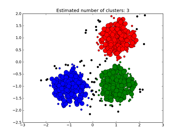
Density Based Clustering - DBSCAN

centers = [[1, 1], [-1, -1], [1, -1]]
X, labels_true = make_blobs(n_samples=750, centers=centers, cluster_std=0.4,
                            random_state=0)
plt.scatter(X[:,0], X[:,1],s=10)

from sklearn.cluster import DBSCAN
from sklearn.preprocessing import StandardScaler
X = StandardScaler().fit_transform(X)

db = DBSCAN(eps=0.3, min_samples=10).fit(X)
core_samples_mask = np.zeros_like(db.labels_, dtype=bool)
core_samples_mask[db.core_sample_indices_] = True
labels = db.labels_

plt.scatter(X[:,0], X[:,1],s=10,c=labels)

Measuring Performance of Clusters衡量聚类的性能

• Two forms of evaluation
• supervised, which uses a ground truth class values for each sample.
  • completeness_score
  • homogeneity_score
• unsupervised, which measures the quality of model itself
  • silhoutte_score
  • calinski_harabaz_score
• 两种评估形式
• 有监督的，它对每个样本使用基本事实类别值。
  • completeness_score
  • homogenity_score
• 无人监督，它衡量模型本身的质量
  • silhoutte_score
  • calinski_harabaz_score

completeness_score

• A clustering result satisfies completeness if all the data points that are members of a given class are elements of the same cluster.
• Accuracy is 1.0 if data belonging to same class belongs to same cluster, even if multiple classes belongs to same cluster
• 如果属于给定类的所有数据点都是同一群集的元素，则群集结果将满足完整性要求
• 如果属于同一类别的数据属于同一群集，则即使多个类别属于同一群集，精度也为1.0

from sklearn.metrics.cluster import completeness_score

completeness_score( labels_true=[10,10,11,11],labels_pred=[1,1,0,0])

1.0

• The acuracy is 1.0 because all the data belonging to same class belongs to same cluster

completeness_score( labels_true=[11,22,22,11],labels_pred=[1,0,1,1])

0.3836885465963443

• The accuracy is .3 because class 1 - [11,22,11], class 2 - [22]

print(completeness_score([10, 10, 11, 11], [0, 0, 0, 0]))

1.0

homogeneity_score

• A clustering result satisfies homogeneity if all of its clusters contain only data points which are members of a single class.

from sklearn.metrics.cluster import homogeneity_score

homogeneity_score([0, 0, 1, 1], [1, 1, 0, 0])

1.0

homogeneity_score([0, 0, 1, 1], [0, 1, 2, 3])

0.9999999999999999

homogeneity_score([0, 0, 0, 0], [1, 1, 0, 0])

1.0

• Same class data is broken into two clusters

silhoutte_score

• The Silhouette Coefficient is calculated using the mean intra-cluster distance (a) and the mean nearest-cluster distance (b) for each sample.
• The Silhouette Coefficient for a sample is (b - a) / max(a, b). To clarify, b is the distance between a sample and the nearest cluster that the sample is not a part of.

Example : Selecting the number of clusters with silhouette analysis on KMeans clustering

from sklearn.datasets import make_blobs
X, Y = make_blobs(n_samples=500,
                  n_features=2,
                  centers=4,
                  cluster_std=1,
                  center_box=(-10.0, 10.0),
                  shuffle=True,
                  random_state=1)

plt.scatter(X[:,0],X[:,1],s=10)

range_n_clusters = [2, 3, 4, 5, 6]
from sklearn.cluster import KMeans
from sklearn.metrics import silhouette_score
for n_cluster in range_n_clusters:
    kmeans = KMeans(n_clusters=n_cluster)
    kmeans.fit(X)
    labels = kmeans.predict(X)
    print (n_cluster, silhouette_score(X,labels))

2 0.7049787496083262
3 0.5882004012129721
4 0.6505186632729437
5 0.5745029081702377
6 0.4544511749648251

• Optimal number of clusters seems to be 2

calinski_harabaz_score

• The score is defined as ratio between the within-cluster dispersion and the between-cluster dispersion.
• 群集的最佳数量似乎是2
• 分数定义为群集内分散度和群集间分散度之间的比率。

from sklearn.metrics import calinski_harabaz_score

for n_cluster in range_n_clusters:
    kmeans = KMeans(n_clusters=n_cluster)
    kmeans.fit(X)
    labels = kmeans.predict(X)
    print (n_cluster, calinski_harabaz_score(X,labels))

2 1604.112286409658
3 1809.991966958033
4 2704.4858735121097
5 2281.933655783649
6 2016.011232059114