经过上一篇文章的学习,我们对于浅层神经网络的学习已经有了初步印象,我们来复习以下:
对于神经网络,我们已经有了神经元的概念:每一个都是一个单独的回归函数罢了
对于从回归学习到浅层神经网络,我们知道添加隐藏层可以提高预测的准确率,并且成功定义了add_layer方法为我们添加节点,快速生成隐藏层
但是我们在浅层神经网络的学习里面的构建隐藏层还是采用了写死的方式,如果说要是想从浅层神经网络改成深层神经网络,则需要对上篇代码继续修改/
深层神经网络
和浅层神经网络不同的是,深层神经网络的隐藏层是可变的,我们可以根据不同的数据源、训练集和数据特征来改变学习策略,以此达到一个比较好的学习效果。
一个两层的深层神经网络结构如下:
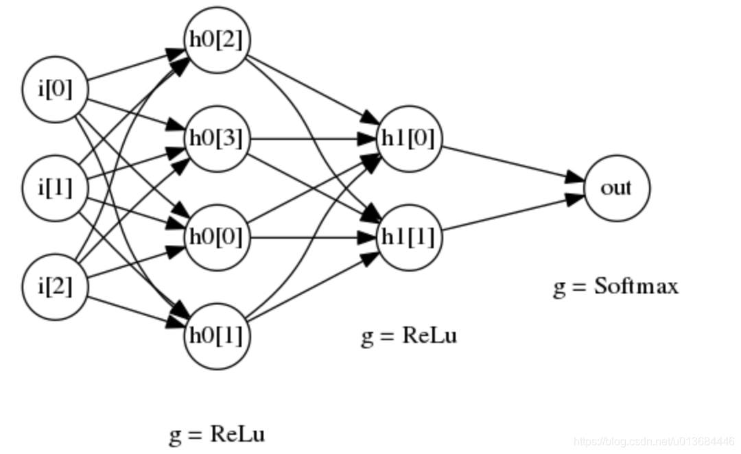
上图所示的是一个具有两层隐藏层的深层神经网络
- 第一个隐藏层有 4 个节点,对应的激活函数为 ReLu 函数
- 第一个隐藏层有 2 个节点,对应的激活函数也是 Relu 函数
- 最后,输出层使用 softmax 函数作为激活函数
那么对于这样的,或者更多的神经网络,我们不可以再用下面的方法:
#浅层

    # 添加隐藏层
    l1 = add_layer(X, 784, 2000, activation_function=tf.nn.relu)
    pre = add_layer(l1, 2000, 10, activation_function=None)  # 输出
而是要先对深层网络的节点做好配置,之后构建可以服用的for循环函数,从而快速搭建
 #深层
 #【重点】规定节点结构
    layer_dims = [784,500,500,10] #结构,结构配置的地方
    layer_count = len(layer_dims)-1 #深度计算不算输入层

    layer_iter = X #初始化输入值,因节点输入层构建需要所以第一层用X,for循环构建神经网络,遍历layer_dims替换X
    for l in range(1,layer_count):
        layer_iter = add_layer(layer_iter,layer_dims[l-1],layer_dims[l],activation_function = tf.nn.relu)
    pre = add_layer(layer_iter,layer_dims[layer_count-1],layer_dims[layer_count],activation_function = None) #输出层节点要用最后一层隐藏层节点数量做输入
我们只需要改变这个构建方法即可,其它方式均可不变,最后得到代码:
#-*- coding:utf-8 -*-
import numpy as np
import matplotlib.pyplot as plt
import tensorflow as tf
from tensorflow.examples.tutorials.mnist import input_data

def add_layer(inputs ,in_size,out_size,activation_function= True):
    #初始化变量
    W = tf.Variable(tf.random_normal([in_size,out_size]))#初始化正态分布,in列,out行,第一层in传入784,第二层传入1000
    b = tf.Variable(tf.zeros([1,out_size])) #偏置量初始化,1列。out行

    Z = tf.matmul(inputs,W)+b #初始化公式,每一层都要有

     #为了防止报错,如果没有传入激活共识,则不作处理
    if activation_function is None:
        outputs = Z
    else:
        outputs = activation_function(Z)

    return outputs
 #构建主函数逻辑
if __name__ == "__main__":
    MNIST = input_data.read_data_sets("./", one_hot=True)
    cost_accum = []

    learning_rate = 0.01
    batch_size = 128
    n_epochs = 22

    X = tf.placeholder(tf.float32, [batch_size, 784])
    Y = tf.placeholder(tf.float32, [batch_size, 10])
    #【重点】规定节点结构
    layer_dims = [784,500,500,10] #结构,结构配置的地方
    layer_count = len(layer_dims)-1 #深度计算不算输入层

    layer_iter = X #初始化输入值,因节点输入层构建需要所以第一层用X,for循环构建神经网络,遍历layer_dims替换X
    for l in range(1,layer_count):
        layer_iter = add_layer(layer_iter,layer_dims[l-1],layer_dims[l],activation_function = tf.nn.relu)
    pre = add_layer(layer_iter,layer_dims[layer_count-1],layer_dims[layer_count],activation_function = None) #输出层节点要用最后一层隐藏层节点数量做输入

    # 添加隐藏层
    # l1 = add_layer(X, 784, 2000, activation_function=tf.nn.relu)
    # pre = add_layer(l1, 2000, 10, activation_function=None)  # 输出
    # w = tf.Variable(tf.random_normal(shape=[784,10], stddev=0.01), name="weights")
    # b = tf.Variable(tf.zeros([1, 10]), name="bias")

    # logits = tf.matmul(X, w) + b

    entropy = tf.nn.softmax_cross_entropy_with_logits(labels=Y, logits=pre)
    loss = tf.reduce_mean(entropy)
    optimizer = tf.train.AdamOptimizer(learning_rate=learning_rate).minimize(loss)
    # optimizer = tf.train.GradientDescentOptimizer(learning_rate=learning_rate).minimize(loss)

    init = tf.global_variables_initializer()

    with tf.Session() as sess:
        sess.run(init)

        n_batches = int(MNIST.train.num_examples/batch_size)
        for i in range(n_epochs):
            for j in range(n_batches):
                X_batch, Y_batch = MNIST.train.next_batch(batch_size)
                loss_ = sess.run([optimizer, loss], feed_dict={ X: X_batch, Y: Y_batch})
                if j==0 :
                    print("Loss of epochs[{0}]: {1}".format(i, loss_))
                cost_accum.append(loss_)


        n_batches = int(MNIST.test.num_examples/batch_size)
        total_correct_preds = 0
        for i in range(n_batches):
            X_batch, Y_batch = MNIST.test.next_batch(batch_size)
            # preds = tf.nn.softmax(tf.matmul(X_batch, w) + b)  # 算预测结果
            preds = sess.run(pre, feed_dict={X: X_batch, Y: Y_batch}) #算预测结果
            correct_preds = tf.equal(tf.argmax(preds, 1), tf.argmax(Y_batch, 1)) #判断预测结果和标准结果
            accuracy = tf.reduce_sum(tf.cast(correct_preds, tf.float32))#先转化判断的字符类型,再降维求和,这样就得到了一大堆压缩后的判断结果
            total_correct_preds += sess.run(accuracy) #之前都是公式,必须要run才有用,然后记录数量


        print("Accuracy {0}".format(total_correct_preds/MNIST.test.num_examples))#判断正确率并输出

    plt.plot(range(len(cost_accum)), cost_accum, 'r')
    plt.title('Logic Regression Cost Curve')
    plt.xlabel('epoch*batch')
    plt.ylabel('loss')
    print('show')
    plt.show()
为了提高代码的复用性质,我将构建+学习部分、绘图部分单独变成了两个方法,得到代码如下:
#-*- coding:utf-8 -*-
import matplotlib.pyplot as plt
import tensorflow as tf
from tensorflow.examples.tutorials.mnist import input_data

def add_layer(inputs ,in_size,out_size,activation_function= True):
    #初始化变量
    W = tf.Variable(tf.random_normal([in_size,out_size]))#初始化正态分布,in列,out行,第一层in传入784,第二层传入1000
    b = tf.Variable(tf.zeros([1,out_size])) #偏置量初始化,1列。out行

    Z = tf.matmul(inputs,W)+b #初始化公式,每一层都要有

     #为了防止报错,如果没有传入激活共识,则不作处理
    if activation_function is None:
        outputs = Z
    else:
        outputs = activation_function(Z)

    return outputs

def draw(cost_accum):
    plt.plot(range(len(cost_accum)), cost_accum, 'r')
    plt.title('Logic Regression Cost Curve')
    plt.xlabel('epoch*batch')
    plt.ylabel('loss')
    print('show')
    plt.show()

def learning(layer_dims,layer_count,layer_iter,input_data):
    for l in range(1,layer_count):
        layer_iter = add_layer(layer_iter,layer_dims[l-1],layer_dims[l],activation_function = tf.nn.relu)
    pre = add_layer(layer_iter,layer_dims[layer_count-1],layer_dims[layer_count],activation_function = None) #输出层节点要用最后一层隐藏层节点数量做输入

    entropy = tf.nn.softmax_cross_entropy_with_logits(labels=Y, logits=pre)
    loss = tf.reduce_mean(entropy)
    optimizer = tf.train.AdamOptimizer(learning_rate=learning_rate).minimize(loss)
    # optimizer = tf.train.GradientDescentOptimizer(learning_rate=learning_rate).minimize(loss)

    init = tf.global_variables_initializer()

    with tf.Session() as sess:
        sess.run(init)

        cost_accum = [] #绘制信息收集
        n_batches = int(input_data.train.num_examples / batch_size)
        for i in range(n_epochs):
            for j in range(n_batches):
                X_batch, Y_batch = input_data.train.next_batch(batch_size)
                loss_ = sess.run([optimizer, loss], feed_dict={X: X_batch, Y: Y_batch})
                if j == 0:
                    print("Loss of epochs[{0}]: {1}".format(i, loss_))
                cost_accum.append(loss_)

        n_batches = int(input_data.test.num_examples / batch_size)
        total_correct_preds = 0
        for i in range(n_batches):
            X_batch, Y_batch = input_data.test.next_batch(batch_size)
            # preds = tf.nn.softmax(tf.matmul(X_batch, w) + b)  # 算预测结果
            preds = sess.run(pre, feed_dict={X: X_batch, Y: Y_batch})  # 算预测结果
            correct_preds = tf.equal(tf.argmax(preds, 1), tf.argmax(Y_batch, 1))  # 判断预测结果和标准结果
            accuracy = tf.reduce_sum(tf.cast(correct_preds, tf.float32))  # 先转化判断的字符类型,再降维求和,这样就得到了一大堆压缩后的判断结果
            total_correct_preds += sess.run(accuracy)  # 之前都是公式,必须要run才有用,然后记录数量

        print("Accuracy {0}".format(total_correct_preds / MNIST.test.num_examples))  # 判断正确率并输出

        draw(cost_accum = cost_accum)

#构建主函数逻辑
if __name__ == "__main__":
    MNIST = input_data.read_data_sets("./", one_hot=True)

    learning_rate = 0.01
    batch_size = 128
    n_epochs = 22

    X = tf.placeholder(tf.float32, [batch_size, 784])
    Y = tf.placeholder(tf.float32, [batch_size, 10])
    #【重点】规定节点结构
    layer_dims = [784,500,500,10] #结构,结构配置的地方
    layer_count = len(layer_dims)-1 #深度计算不算输入层
    layer_iter = X #初始化输入值,因节点输入层构建需要所以第一层用X,for循环构建神经网络,遍历layer_dims替换X

    learning(layer_dims =layer_dims,layer_count = layer_count,layer_iter = layer_iter,input_data = MNIST)
经过训练22次之后,结果为:
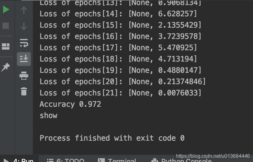
此外,我们可以在主函数当中调整配置,来做一下对比实验:调整layer_dims = [784,800,200,10]
来观察实验结果
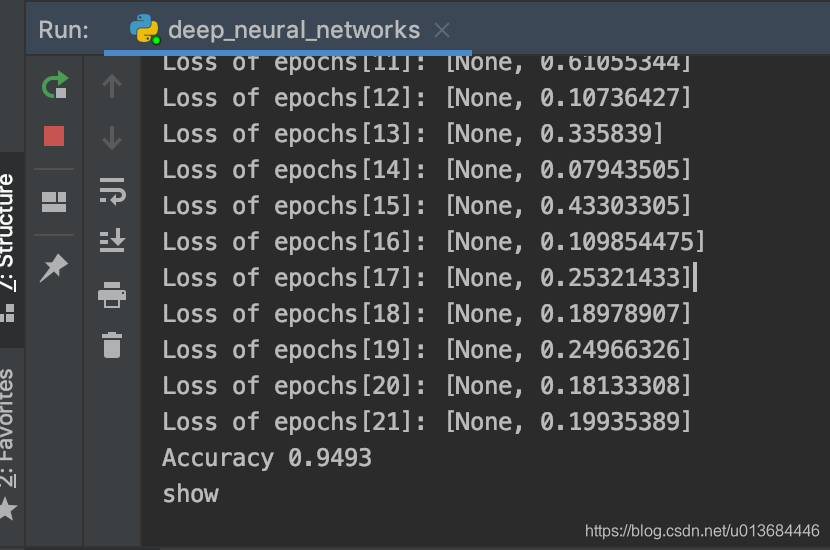
调整layer_dims = [784,200,800,10]
来观察实验结果
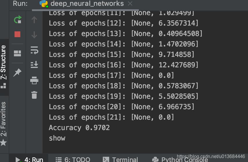
可见神经元结构对于学习效果是有显著影响的!
你也可以多去尝试新得到算法、结构,这就是算法和结构的优化啦~
下一篇文章,我们将走进被神化的算法:卷积神经网络,看看他和我们有什么不同,又怎样的独特效果。
