文章目录
前言
该曲线拟合的例子来源于高翔,但是他的版本首先是g2o过旧,这里面包含了新旧版本的g2o中曲线拟合的实现,其次是不适用于现在的版本,而且存在使用Opencv的依赖项。本次实现不需要Opencv的依赖项,不过看个人喜好,我在里面进行了注释。
代码
目前已经放在github上。
github地址:https://github.com/tanqiwei/g2oProject
代码说明
代码中分新旧版本,分为两个文件夹,g2o_source_github保存的是我所使用的新旧版本的g2o的github源码(已解压或曾编译),g2o_project保存我目前的项目。
曲线拟合
问题描述
假设我们有一系列的点,我们假设它们满足于下面的公式:
但是这些点受到高斯噪声影响,使得不完全满足上述的式子。故而我们需要做的是曲线拟合操作,使得估计出来好的 构建出来的下面的方程式:
使得最小化
这实际上是最小二乘问题。
流程步骤
安装第二篇博文阅读的g2o的文档,尤其是说明2D SLAM之后,大概你可以归纳几个步骤:
- 问题建模
- 定义顶点和边的实现类型
- 误差函数的设计
- 实现
问题建模
我们把这个问题正如高翔在SLAM十四讲中123页所构建的模型。
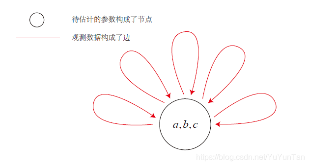
要估计的部分构成一个顶点,所有的边都与该顶点相连。这是一个超图问题。还记得超图的定义么,目前我的理解是,只有一条边连接不是两个顶点的图便是g2o所定义的超图。
那么我们可以构建一个顶点,多个边,而这个边是一元边,顶点的类型的数据是三个数值构成的量,可以用Eigen3::Vector3d表示。在第二篇博文中的“优化问题的表示”则描述了边和顶点的g2o支持类型,我们需要做的则是扩展。
顶点的定义
我们需要继承的是BaseVertex。BaseVertex的两个模板,第一个是模板的最小维度(比如三维旋转空间是3),第二个是表达估计的内部类型(比如四元数)。这里采用高翔的实现,用Vector3d去保存和更新顶点。根据第二篇博文的“优化问题的表示”那里说明,我们需要定义和实现setToOriginImpl()方法和oplusImpl(const double* update)方法。
class CurveFittingVetex: public g2o::BaseVertex<3,Eigen::Vector3d>
{
    // BaseVertex的两个模板,第一个是模板的最小维度(比如三维旋转空间是3),第二个是表达估计的内部类型(比如四元数),
public:
    // Eigen的使用时内存对齐
    EIGEN_MAKE_ALIGNED_OPERATOR_NEW
    virtual void setToOriginImpl();
    virtual void oplusImpl(const double* update);
    // 读写函数
    virtual bool read(std::istream &is);
    virtual bool write(std::ostream &os) const ;
};
这是实现的cpp
//
// Created by tqw on 18-12-26.
//
#include "commonBased.h"
#include "CurveFittingVetex.h"

void CurveFittingVetex::setToOriginImpl()  // 重置
{// 顶点内部状态初始值
    _estimate << 0,0,0;
}

void CurveFittingVetex::oplusImpl(const double *update) // 该方法应该应用一个增量用于更新估计参数$\oplus$
{
    _estimate += Eigen::Vector3d(update);
}

bool CurveFittingVetex::read(std::istream &is)
{
    is >> _estimate[0] >> _estimate[1] >> _estimate[2];
    return true;
}
bool CurveFittingVetex::write(std::ostream &os) const
{
    os <<  _estimate[0] << _estimate[1] << _estimate[2];
    return os.good();
}
边的定义
由于是一元边,只有一个顶点相连。所以继承只能是BaseUnaryEdge,具体情况具体分析,目前是一元边。
class CurveFittingEdge: public g2o::BaseUnaryEdge<1,double,CurveFittingVetex>
{
    //   一元超边,即只连接一个顶点,要给出三个,一个是维度,一个是变量类型,一个是连接的顶点类型
public:
    EIGEN_MAKE_ALIGNED_OPERATOR_NEW
    // 构造函数
    CurveFittingEdge (double x):g2o::BaseUnaryEdge<1,double,CurveFittingVetex>(),_x (x) {};
    // 计算曲线模型误差
    void computeError();
    //存取
    bool read(std::istream& is);
    bool write(std::ostream& os) const;

public:
    double _x;//x值,y值为_measurement
};
这是实现的cpp
一元超边,超边存储的节点为VertexContainer类型,你可以把它当成一个数组,取第一个就是0,对于一元边来说,这就是它的连接的边。而_error(0,0) 是Eigen::Matrix<number_t, D, 1, Eigen::ColMajor>类型,传入的时候已经指明D=1,所以是一行一列的矩阵(只有一个元素)。
#include "CurveFittingEdge.h"

void CurveFittingEdge::computeError()
{
    // 一元超边,超边存储的节点为VertexContainer类型,你可以把它当成一个数组,取第一个就是0,对于一元边来说,这就是它的
    // 连接的边
    const CurveFittingVetex *v = static_cast<const CurveFittingVetex*>(_vertices[0]);
    const Eigen::Vector3d abc = v->estimate();
    // _error是传入时定义的误差ErrorVector,维度D是构建CurveFittingEdge已经定义,必然是个向量,只不过是Eigen::Matrix的_Cols为1
    _error(0,0) = _measurement-std::exp(abc[0]*pow(_x,2)+abc[1]*_x+abc[2]);// y-f(x)=error
}
bool CurveFittingEdge::read(std::istream &is)
{
    is >> _x;
    return true;
}
bool CurveFittingEdge::write(std::ostream &os) const
{
    os << _x;
    return os.good();
}
误差函数的设计
我们在上面已经说明了,误差定义为 ,这在代码中有实现,比如:
_error(0,0) = _measurement-std::exp(abc[0]*pow(_x,2)+abc[1]*_x+abc[2]);// y-f(x)=error
具体实现
旧版本的g2o实现
我们算法的流程主要如下所示:
/**
 * 这是关于旧版本即SLAM十四讲的g2o版本进行的代码编写和注释
 * 旧版本和新版本在用法上不一定一样
 */

#include "commonBased.h"
#include "CurveFittingVetex.h"
#include "CurveFittingEdge.h"

int main()
{
    std::cout << "====================================================" << std::endl;
    std::cout << "\t\t\t\t这是关于曲线拟合的例子" << std::endl;
    std::cout << "====================================================" << std::endl;
    std::cout << "\t\t\t\t anthor:YuYunTan" << std::endl;
    std::cout << "====================================================" << std::endl;
    std::cout << "\t\t\t\treference:gaoxiang" << std::endl;
    std::cout << "====================================================" << std::endl;

    // 真实参数,假设曲线是f(x)=a*x^2+b*x+c,真实情况下应该是f(x)=x^2+2*x+1
    double a = 1.0,b=2.0,c =1.0;
    int N = 100;// 数据点的数量
    double w_sigma = 1.0;// 噪声的方差Sigma
    //cv::RNG rng;// opencv随机数产生器,如果要使用opencv的高斯0均值随机数发生器,请在commonBased引入[将注释取消即可]
    double abc[3] = {0,0,0};// abc参数的估计值

    std::vector<double> x_data,y_data;//保存随机数的值,即模拟真实点的情况
    std::cout << "\t\t\t\t generating data:" << std::endl;
    std::cout << "====================================================" << std::endl;
    for(auto i=0;i<N;i++)
    {
        double  x = i/100.0;
        x_data.push_back(x);
        y_data.push_back(
          //exp(a*x*x+b*x+c)+rng.gaussian(w_sigma)
          exp(a*pow(x,2)+b*x+c)+g2o::Sampler::gaussRand(0,w_sigma)// 采用G2O的随机发生器
        );

        std::cout << x_data[i] << " " << y_data[i] << std::endl;
    }
    std::cout << "====================================================" << std::endl;
    std::cout << "\t\t\t\t       构建图:" << std::endl;
    // 构建g2o图优化问题

    // 矩阵块: 每个误差项优化维度为3,误差值维度为1
    /**
     * 要优化的变量是(a,b,c),这个变量含有三个维度,在eigen3中最好的存储方式是Eigen:Vector3d
     * 误差是一维的,因为结果值是一维度的.两者相减还是一个维度
     */
    typedef g2o::BlockSolver<g2o::BlockSolverTraits<3,1>> Block;
    Block::LinearSolverType* linearSolver = new g2o::LinearSolverDense<Block::PoseMatrixType>();
    Block* solver_ptr = new Block(linearSolver);
    // 梯度下降方法:GN,LM,Dogleg中选
    g2o::OptimizationAlgorithmLevenberg* solver = new g2o::OptimizationAlgorithmLevenberg(solver_ptr);
    // GN
    //g2o::OptimizationAlgorithmGaussNewton* solver = new g2o::OptimizationAlgorithmGaussNewton(solver_ptr);
    // Dogleg
    //g2o::OptimizationAlgorithmDogleg* solver = new g2o::OptimizationAlgorithmDogleg(solver_ptr);
    // 图模型
    g2o::SparseOptimizer optimizer;
    optimizer.setAlgorithm(solver);// 设置求解器
    optimizer.setVerbose(true);// 打开调试输出

    // 对图中添加顶点
    CurveFittingVetex* v = new CurveFittingVetex();
    v->setEstimate(Eigen::Vector3d(0,0,0));
    v->setId(0);
    optimizer.addVertex(v);
    // 全程只有一个顶点,该顶点用多条一元边连接
    for(int i=0;i<N;i++)
    {
        CurveFittingEdge *edge = new CurveFittingEdge(x_data[i]);
        edge->setId(i);// 边的编号
        edge->setVertex(0,v);//设置超边的第几个顶点是什么顶点,目前只有一个顶点
        edge->setMeasurement(y_data[i]);//设置观测值
        edge->setInformation(Eigen::Matrix<double ,1,1>::Identity()*1/(w_sigma*w_sigma));//信息矩阵是协方差的逆,1/sigma^2
        optimizer.addEdge(edge);// 图中加入顶点

    }
    std::cout << "\t\t\t\t     构建完成" << std::endl;
    std::cout << "====================================================" << std::endl;
    std::cout << "\t\t\t\t start optimization" << std::endl;
    std::chrono::steady_clock::time_point t1 = std::chrono::steady_clock::now();
    optimizer.initializeOptimization();
    optimizer.optimize(100);//设置最大迭代次数
    std::chrono::steady_clock::time_point t2 = std::chrono::steady_clock::now();
    std::chrono::duration<double> time_used = std::chrono::duration_cast<std::chrono::duration<double>> (t2-t1);
    std::cout << "====================================================" << std::endl;
    std::cout << "\t\t solve time cost = "<< time_used.count() << "seconds" <<std::endl;
    std::cout << "====================================================" << std::endl;
    // 输出优化值
    Eigen::Vector3d abc_estimate = v->estimate();
    std::cout << "\t\t estimated model:" << abc_estimate.transpose() << std::endl;

    return 0;
}
新版本的g2o实现
主要是在求解器的生成上,使用了移动构造和右值引用以及智能指针。
/**
 * 这是关于新版本即github上2018年12月21日的g2o版本进行的代码编写和注释
 * 旧版本和新版本在用法上不一定一样
 */


#include "commonBased.h"
#include "CurveFittingVetex.h"
#include "CurveFittingEdge.h"


int main()
{
    std::cout << "====================================================" << std::endl;
    std::cout << "\t\t\t\t这是关于曲线拟合的例子" << std::endl;
    std::cout << "====================================================" << std::endl;
    std::cout << "\t\t\t\t anthor:YuYunTan" << std::endl;
    std::cout << "====================================================" << std::endl;
    std::cout << "\t\t\t\treference:gaoxiang" << std::endl;
    std::cout << "====================================================" << std::endl;

    // 真实参数,假设曲线是f(x)=a*x^2+b*x+c,真实情况下应该是f(x)=x^2+2*x+1
    double a = 1.0,b=2.0,c =1.0;
    int N = 100;// 数据点的数量
    double w_sigma = 1.0;// 噪声的方差Sigma
    //cv::RNG rng;// opencv随机数产生器,如果要使用opencv的高斯0均值随机数发生器,请在commonBased引入[将注释取消即可]
    double abc[3] = {0,0,0};// abc参数的估计值

    std::vector<double> x_data,y_data;//保存随机数的值,即模拟真实点的情况
    std::cout << "\t\t\t\t generating data:" << std::endl;
    std::cout << "====================================================" << std::endl;
    for(auto i=0;i<N;i++)
    {
        double  x = i/100.0;
        x_data.push_back(x);
        y_data.push_back(
                //exp(a*x*x+b*x+c)+rng.gaussian(w_sigma)
                exp(a*pow(x,2)+b*x+c)+g2o::Sampler::gaussRand(0,w_sigma)// 采用G2O的随机发生器
        );

        std::cout << x_data[i] << " " << y_data[i] << std::endl;
    }
    std::cout << "====================================================" << std::endl;
    std::cout << "\t\t\t\t       构建图:" << std::endl;
    // 构建g2o图优化问题

    // 矩阵块: 每个误差项优化维度为3,误差值维度为1
    /**
     * 要优化的变量是(a,b,c),这个变量含有三个维度,在eigen3中最好的存储方式是Eigen:Vector3d
     * 误差是一维的,因为结果值是一维度的.两者相减还是一个维度
     */
    // 新版本在构建上进行了更改
    typedef g2o::BlockSolver<g2o::BlockSolverTraits<3,1>> Block;
    auto linearSolver = g2o::make_unique<g2o::LinearSolverDense<Block::PoseMatrixType>>();// 使用了智能指针,而非指针类型
    auto solver_ptr = g2o::make_unique<Block>(std::move(linearSolver));// 改成了使用移动构造函数构建求解器
    // 梯度下降方法:GN,LM,Dogleg中选
    g2o::OptimizationAlgorithmLevenberg* solver = new g2o::OptimizationAlgorithmLevenberg(std::move(solver_ptr));
    // GN
    //g2o::OptimizationAlgorithmGaussNewton* solver = new g2o::OptimizationAlgorithmGaussNewton(std::move(solver_ptr));
    // Dogleg
    //g2o::OptimizationAlgorithmDogleg* solver = new g2o::OptimizationAlgorithmDogleg(std::move(solver_ptr));
    // 图模型
    g2o::SparseOptimizer optimizer;
    optimizer.setAlgorithm(solver);// 设置求解器
    optimizer.setVerbose(true);// 打开调试输出

    // 对图中添加顶点
    CurveFittingVetex* v = new CurveFittingVetex();
    v->setEstimate(Eigen::Vector3d(0,0,0));
    v->setId(0);
    optimizer.addVertex(v);
    // 全程只有一个顶点,该顶点用多条一元边连接
    for(int i=0;i<N;i++)
    {
        CurveFittingEdge *edge = new CurveFittingEdge(x_data[i]);
        edge->setId(i);// 边的编号
        edge->setVertex(0,v);//设置超边的第几个顶点是什么顶点,目前只有一个顶点
        edge->setMeasurement(y_data[i]);//设置观测值
        edge->setInformation(Eigen::Matrix<double ,1,1>::Identity()*1/(w_sigma*w_sigma));//信息矩阵是协方差的逆,1/sigma^2
        optimizer.addEdge(edge);// 图中加入顶点

    }
    std::cout << "\t\t\t\t     构建完成" << std::endl;
    std::cout << "====================================================" << std::endl;
    std::cout << "\t\t\t\t start optimization" << std::endl;
    std::chrono::steady_clock::time_point t1 = std::chrono::steady_clock::now();
    optimizer.initializeOptimization();
    optimizer.optimize(100);//设置最大迭代次数
    std::chrono::steady_clock::time_point t2 = std::chrono::steady_clock::now();
    std::chrono::duration<double> time_used = std::chrono::duration_cast<std::chrono::duration<double>> (t2-t1);
    std::cout << "====================================================" << std::endl;
    std::cout << "\t\t solve time cost = "<< time_used.count() << "seconds" <<std::endl;
    std::cout << "====================================================" << std::endl;
    // 输出优化值
    Eigen::Vector3d abc_estimate = v->estimate();
    std::cout << "\t\t estimated model:" << abc_estimate.transpose() << std::endl;
    return 0;
}
我们的输出如下所示,为了边幅问题,我只展示新版本g2o的输出:
====================================================
				这是关于曲线拟合的例子
====================================================
				 anthor:YuYunTan
====================================================
				reference:gaoxiang
====================================================
				 generating data:
====================================================
0 2.37296
0.01 3.41448
0.02 3.9895
0.03 3.30644
0.04 5.2303
0.05 3.23683
0.06 4.46305
0.07 3.45031
0.08 3.51076
0.09 2.95948
0.1 4.59765
0.11 1.89857
0.12 3.89844
0.13 4.05831
0.14 4.6485
0.15 5.30929
0.16 4.73513
0.17 3.02651
0.18 3.16154
0.19 4.68424
0.2 3.91599
0.21 3.60526
0.22 4.72053
0.23 5.87669
0.24 6.73519
0.25 4.20824
0.26 5.62264
0.27 5.18107
0.28 6.13236
0.29 3.90759
0.3 4.52046
0.31 6.57398
0.32 5.20906
0.33 6.21616
0.34 7.36287
0.35 6.29002
0.36 7.26244
0.37 7.31245
0.38 7.93896
0.39 7.49406
0.4 5.60134
0.41 6.36557
0.42 6.04772
0.43 7.04742
0.44 6.45343
0.45 7.5893
0.46 6.33141
0.47 10.2936
0.48 7.9647
0.49 8.50427
0.5 8.49451
0.51 8.28341
0.52 10.5486
0.53 10.6653
0.54 11.2207
0.55 11.0827
0.56 10.8602
0.57 12.4138
0.58 12.365
0.59 13.8104
0.6 12.1146
0.61 14.675
0.62 15.324
0.63 13.0292
0.64 14.3658
0.65 15.9836
0.66 14.3987
0.67 15.6273
0.68 18.4271
0.69 18.3935
0.7 18.6976
0.71 18.6793
0.72 19.2327
0.73 20.2861
0.74 19.391
0.75 20.0922
0.76 21.0915
0.77 21.8079
0.78 23.9708
0.79 25.2857
0.8 26.0174
0.81 26.8393
0.82 26.8545
0.83 30.9203
0.84 29.4622
0.85 31.5744
0.86 32.8773
0.87 32.5152
0.88 34.077
0.89 33.6634
0.9 36.1023
0.91 37.964
0.92 41.5879
0.93 42.586
0.94 42.0306
0.95 46.4002
0.96 45.7122
0.97 47.6634
0.98 50.6537
0.99 51.2023
====================================================
				       构建图:
				     构建完成
====================================================
				 start optimization
iteration= 0	 chi2= 29756.413204	 time= 0.00352656	 cumTime= 0.00352656	 edges= 100	 schur= 0	 lambda= 699.050633	 levenbergIter= 7
iteration= 1	 chi2= 13229.425289	 time= 0.00284606	 cumTime= 0.00637262	 edges= 100	 schur= 0	 lambda= 1864.135020	 levenbergIter= 3
iteration= 2	 chi2= 7036.389558	 time= 0.00273867	 cumTime= 0.00911129	 edges= 100	 schur= 0	 lambda= 1242.756680	 levenbergIter= 1
iteration= 3	 chi2= 262.481389	 time= 0.00267204	 cumTime= 0.0117833	 edges= 100	 schur= 0	 lambda= 414.252227	 levenbergIter= 1
iteration= 4	 chi2= 108.202716	 time= 0.00289397	 cumTime= 0.0146773	 edges= 100	 schur= 0	 lambda= 138.084076	 levenbergIter= 1
iteration= 5	 chi2= 105.779911	 time= 0.0029456	 cumTime= 0.0176229	 edges= 100	 schur= 0	 lambda= 46.028025	 levenbergIter= 1
iteration= 6	 chi2= 104.119902	 time= 0.00294632	 cumTime= 0.0205692	 edges= 100	 schur= 0	 lambda= 15.342675	 levenbergIter= 1
iteration= 7	 chi2= 102.894716	 time= 0.00325897	 cumTime= 0.0238282	 edges= 100	 schur= 0	 lambda= 5.114225	 levenbergIter= 1
iteration= 8	 chi2= 102.607436	 time= 0.0030197	 cumTime= 0.0268479	 edges= 100	 schur= 0	 lambda= 1.704742	 levenbergIter= 1
iteration= 9	 chi2= 102.591184	 time= 0.00294795	 cumTime= 0.0297958	 edges= 100	 schur= 0	 lambda= 0.568247	 levenbergIter= 1
iteration= 10	 chi2= 102.590970	 time= 0.00289023	 cumTime= 0.0326861	 edges= 100	 schur= 0	 lambda= 0.378831	 levenbergIter= 1
iteration= 11	 chi2= 102.590970	 time= 0.00277191	 cumTime= 0.035458	 edges= 100	 schur= 0	 lambda= 0.252554	 levenbergIter= 1
iteration= 12	 chi2= 102.590970	 time= 0.00253844	 cumTime= 0.0379964	 edges= 100	 schur= 0	 lambda= 0.168370	 levenbergIter= 1
iteration= 13	 chi2= 102.590970	 time= 0.0027626	 cumTime= 0.040759	 edges= 100	 schur= 0	 lambda= 0.112246	 levenbergIter= 1
iteration= 14	 chi2= 102.590970	 time= 0.00356865	 cumTime= 0.0443277	 edges= 100	 schur= 0	 lambda= 30130904.265572	 levenbergIter= 7
====================================================
		 solve time cost = 0.0471035seconds
====================================================
		 estimated model:1.12835 1.78695 1.08486
总结
目前为止,对于g2o的新旧版本主要体现在求解器的初始化上,大体上在使用流程和以前相差不大。
