这个图描述神经网络挺形象的

keras
搭建一个神经网络
增加各个层
compiling:compile
train:fit
predict:predict
evaluate loss:evaluate
sequence这里比较方便一点
以输入为2,输出层只有一层的为例

# Import the Sequential model and Dense layer
from keras.models import Sequential
from keras.layers import Dense

# Create a Sequential model
model = Sequential()

# Add an input layer and a hidden layer with 10 neurons
model.add(Dense(10, input_shape=(2,), activation="relu"))

# Add a 1-neuron output layer
model.add(Dense(1))

# Summarise your model
model.summary()
一个比较完整的栗子
# Instantiate a Sequential model
model = Sequential()

# Add a Dense layer with 50 neurons and an input of 1 neuron
model.add(Dense(50, input_shape=(1,), activation='relu'))

# Add two Dense layers with 50 neurons and relu activation
model.add(Dense(50, activation='relu'))
model.add(Dense(50, activation='relu'))

# End your model with a Dense layer and no activation
model.add(Dense(1))

# Compile your model
model.compile(optimizer = 'adam', loss = 'mse')

print("Training started..., this can take a while:")

# Fit your model on your data for 30 epochs
model.fit(time_steps, y_positions, epochs = 30)

# Evaluate your model
print("Final lost value:",model.evaluate(time_steps, y_positions))

# Predict the twenty minutes orbit
twenty_min_orbit = model.predict(np.arange(-10, 11))

# Plot the twenty minute orbit
plot_orbit(twenty_min_orbit)
binary classification
那输出的dense层的激活函数是sigmoid就可以了
# Import the sequential model and dense layer
from keras.models import Sequential
from keras.layers import Dense

# Create a sequential model
model = Sequential()

# Add a dense layer
model.add(Dense(1, input_shape=(4,), activation='sigmoid'))

# Compile your model
model.compile(loss='binary_crossentropy', optimizer='sgd', metrics=['accuracy'])

# Display a summary of your model
model.summary()


# Train your model for 20 epochs,假设这里划分好了数据集
model.fit(X_train, y_train, epochs=20)

# Evaluate your model accuracy on the test set
accuracy = model.evaluate(X_test, y_test)[1]

# Print accuracy
print('Accuracy:',accuracy)
Multi-class classification
多分类的话,就是输出的激活函数不是sigmoid了,而是softmax了
所以写一个多分类的流程
就是
定义输入层和隐藏层
定义更多的隐藏层
定义输出层,输出层的结点数量大于一
demo
定义一个含有三个隐藏层神经网络,输出为4分类
# Instantiate a sequential model
model = Sequential()

# Add 3 dense layers of 128, 64 and 32 neurons each
model.add(Dense(128, input_shape=(2,), activation='relu'))
model.add(Dense(64, activation='relu'))
model.add(Dense(32, activation='relu'))

# Add a dense layer with as many neurons as competitors
model.add(Dense(4, activation='softmax'))

# Compile your model using categorical_crossentropy loss
model.compile(loss='categorical_crossentropy',
              optimizer='adam',
              metrics=['accuracy'])


# Train your model on the training data for 200 epochs
model.fit(coord_train, competitors_train, epochs=200)

# Evaluate your model accuracy on the test data
accuracy = model.evaluate(coord_test, competitors_test)[1]

# Print accuracy
print('Accuracy:', accuracy)
编码形式
labelcoder
# Transform into a categorical variable
darts.competitor = pd.Categorical(darts.competitor)

# Assign a number to each category (label encoding)
darts.competitor = darts.competitor.cat.codes

# Print the label encoded competitors
print('Label encoded competitors: \n',darts.competitor.head())
<script.py> output:
    Label encoded competitors:
     0    2
    1    3
    2    1
    3    0
    4    2
    Name: competitor, dtype: int8
one hot
# Transform into a categorical variable
darts.competitor = pd.Categorical(darts.competitor)

# Assign a number to each category (label encoding)
darts.competitor = darts.competitor.cat.codes

# Import to_categorical from keras utils module
from keras.utils import to_categorical

# Use to_categorical on your labels
coordinates = darts.drop(['competitor'], axis=1)
competitors = to_categorical(darts.competitor)

# Now print the to_categorical() result
print('One-hot encoded competitors: \n',competitors)
Multi-label classification
dense的结点不是1了,而是大于1的,激活函数还是sigmoid
# Instantiate a Sequential model
model = Sequential()

# Add a hidden layer of 64 neurons and a 20 neuron's input
model.add(Dense(64, input_shape=(20,), activation='relu'))

# Add an output layer of 3 neurons with sigmoid activation
model.add(Dense(3, activation='sigmoid'))

# Compile your model with adam and binary crossentropy loss
model.compile(optimizer='adam',
              loss='binary_crossentropy',
              metrics=['accuracy'])

model.summary()
# Train for 100 epochs using a validation split of 0.2
model.fit(sensors_train, parcels_train, epochs=100, validation_split=0.2)

# Predict on sensors_test and round up the predictions
preds = model.predict(sensors_test)
preds_rounded = np.round(preds)

# Print rounded preds
print('Rounded Predictions: \n', preds_rounded)

# Evaluate your model's accuracy on the test data
accuracy = model.evaluate(sensors_test, parcels_test)[1]

# Print accuracy
print('Accuracy:', accuracy)
Keras callbacks
回调函数使用
回调函数是一个函数的合集,会在训练的阶段中所使用。你可以使用回调函数来查看训练模型的内在状态和统计。你可以传递一个列表的回调函数(作为 callbacks 关键字参数)到 Sequential 或 Model 类型的 .fit() 方法。在训练时,相应的回调函数的方法就会被在各自的阶段被调用。keras.cn
在每个training/epoch/batch结束时,如果我们想执行某些任务,例如模型缓存、输出日志、计算当前的auc等等,Keras中的callback就派上用场了。
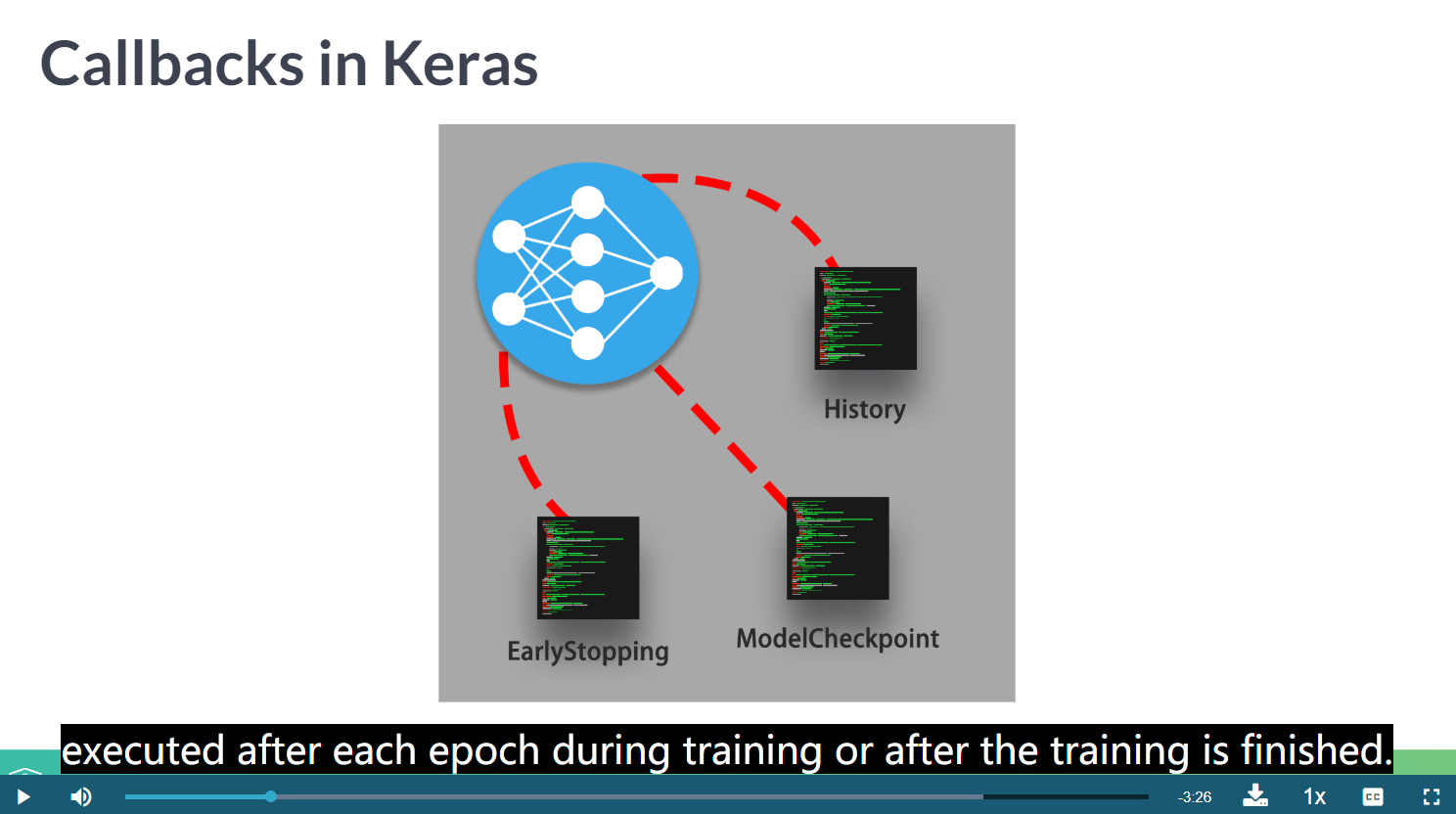
callbacks可以用来做这些事情:
模型断点续训:保存当前模型的所有权重
提早结束:当模型的损失不再下降的时候就终止训练,当然,会保存最优的模型。
动态调整训练时的参数,比如优化的学习速度。
等等
earlystopping和modelcheckpoint抄书侠
import keras
# Callbacks are passed to the model fit the `callbacks` argument in `fit`,
# which takes a list of callbacks. You can pass any number of callbacks.
callbacks_list = [
  # This callback will interrupt training when we have stopped improving
  keras.callbacks.EarlyStopping(
  # This callback will monitor the validation accuracy of the model
  monitor='acc',
  # Training will be interrupted when the accuracy
  # has stopped improving for *more* than 1 epochs (i.e. 2 epochs)
  patience=1,
  ),
  # This callback will save the current weights after every epoch
  keras.callbacks.ModelCheckpoint(
  filepath='my_model.h5', # Path to the destination model file
  # The two arguments below mean that we will not overwrite the
  # model file unless `val_loss` has improved, which
  # allows us to keep the best model every seen during training.
  monitor='val_loss',
  save_best_only=True,
  )
]
# Since we monitor `acc`, it should be part of the metrics of the model.
model.compile(optimizer='rmsprop', loss='binary_crossentropy', metrics=['acc'])
# Note that since the callback will be monitor validation accuracy,
# we need to pass some `validation_data` to our call to `fit`.
model.fit(x, y,
  epochs=10,
  batch_size=32,
  callbacks=callbacks_list,
  validation_data=(x_val, y_val))
monitor为选择的检测指标,我们这里选择检测'acc'识别率为指标,patience就是我们能让训练停止变好多少epochs才终止训练,这里选择了1,而modelcheckpoint就起到了存储最优的模型的作用,filepath为我们存储的位置和模型名称,以.h5为后缀,monitor为检测的指标,这里我们检测验证集里面的成功率,save_best_only代表我们只保存最优的训练结果。
而validation_data就是给定的验证集数据。
学习率减少callback抄书侠
callbacks_list = [
  keras.callbacks.ReduceLROnPlateau(
  # This callback will monitor the validation loss of the model
  monitor='val_loss',
  # It will divide the learning by 10 when it gets triggered
  factor=0.1,
  # It will get triggered after the validation loss has stopped improving
  # for at least 10 epochs
  patience=10,
  )
]# Note that since the callback will be monitor validation loss,
# we need to pass some `validation_data` to our call to `fit`.
model.fit(x, y,
  epochs=10,
  batch_size=32,
  callbacks=callbacks_list,
  validation_data=(x_val, y_val))
翻译一下,就是如果连续10个批次,val_loss不再下降,就把学习率弄到原来的0.1倍。
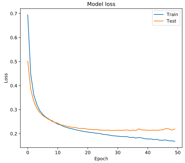
history callback
# Train your model and save its history
history = model.fit(X_train, y_train, epochs = 50,
validation_data=(X_test, y_test))
# Plot train vs test loss during training
plot_loss(history.history['loss'], history.history['val_loss'])
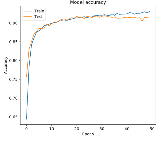
# Plot train vs test accuracy during training
plot_accuracy(history.history['acc'], history.history['val_acc'])
Early stopping your model
The early stopping callback is useful since it allows for you to stop the model training if it no longer improves after a given number of epochs. To make use of this functionality you need to pass the callback inside a list to the model's callback parameter in the .fit() method.
# Import the early stopping callback
from keras.callbacks import EarlyStopping

# Define a callback to monitor val_acc
monitor_val_acc = EarlyStopping(monitor='val_acc',
                                patience=5)

# Train your model using the early stopping callback
model.fit(X_train, y_train,
          epochs=1000, validation_data=(X_test, y_test),
          callbacks=[monitor_val_acc])
EarlyStopping and ModelCheckpoint callbacks
当验证集的误差不再发生变化的时候,停止迭代,并且保存模型为hdf5格式
# Import the EarlyStopping and ModelCheckpoint callbacks
from keras.callbacks import EarlyStopping, ModelCheckpoint

# Early stop on validation accuracy
monitor_val_acc = EarlyStopping(monitor = 'val_acc', patience = 3)

# Save the best model as best_banknote_model.hdf5
modelCheckpoint = ModelCheckpoint('best_banknote_model.hdf5', save_best_only = True)

# Fit your model for a stupid amount of epochs
history = model.fit(X_train, y_train,
                    epochs = 10000000,
                    callbacks = [monitor_val_acc, modelCheckpoint],
                    validation_data = (X_test, y_test))
模型的保存方式
h5格式
Learning curves
学习曲线
查看损失函数的curve和accuary的curve
# Instantiate a Sequential model
model = Sequential()

# Input and hidden layer with input_shape, 16 neurons, and relu
model.add(Dense(16, input_shape = (64,), activation = 'relu'))

# Output layer with 10 neurons (one per digit) and softmax
model.add(Dense(10, activation = 'softmax'))

# Compile your model
model.compile(optimizer = 'adam', loss = 'categorical_crossentropy', metrics = ['accuracy'])

# Test if your model works and can process input data
print(model.predict(X_train))

# 这里划分数据集的方式是通用的,不过这个是留出法

# Train your model for 60 epochs, using X_test and y_test as validation data
history = model.fit(X_train, y_train, epochs=60, validation_data=(X_test, y_test), verbose=0)

# Extract from the history object loss and val_loss to plot the learning curve
plot_loss(history.history['loss'], history.history['val_loss'])
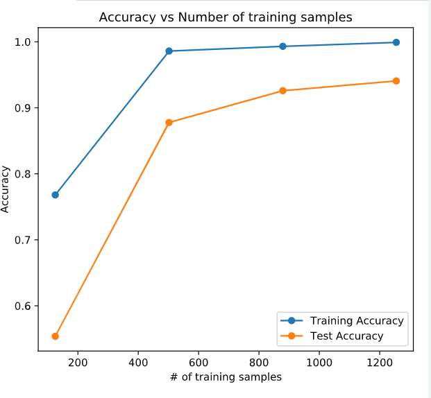
for size in training_sizes:
  	# Get a fraction of training data (we only care about the training data)
    X_train_frac, y_train_frac = X_train[:size], y_train[:size]

    # Reset the model to the initial weights and train it on the new data fraction
    model.set_weights(initial_weights)
    model.fit(X_train_frac, y_train_frac, epochs = 50, callbacks = [early_stop])

    # Evaluate and store the train fraction and the complete test set results
    train_accs.append(model.evaluate(X_train_frac, y_train_frac)[1])
    test_accs.append(model.evaluate(X_test, y_test)[1])

# Plot train vs test accuracies
plot_results(train_accs, test_accs)
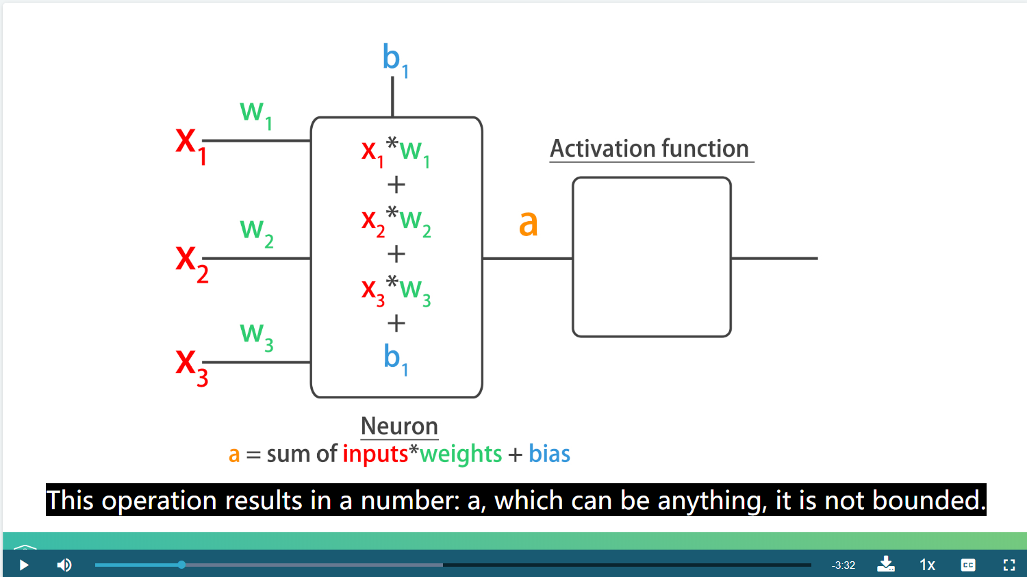
激活函数
神经网络的内部就是一堆的数相乘,求和的过程,这个图很形象了
Batch size and batch normalization
分批的尺寸和每批的正则化
批量标准化层 (Ioffe and Szegedy, 2014)。
在每一个批次的数据中标准化前一层的激活项, 即,应用一个维持激活项平均值接近 0,标准差接近 1 的转换。
# Import batch normalization from keras layers
from keras.layers import BatchNormalization

# Build your deep network
batchnorm_model = Sequential()
batchnorm_model.add(Dense(50, input_shape=(64,), activation='relu', kernel_initializer='normal'))
batchnorm_model.add(BatchNormalization())
batchnorm_model.add(Dense(50, activation='relu', kernel_initializer='normal'))
batchnorm_model.add(BatchNormalization())
batchnorm_model.add(Dense(50, activation='relu', kernel_initializer='normal'))
batchnorm_model.add(BatchNormalization())
batchnorm_model.add(Dense(10, activation='softmax', kernel_initializer='normal'))

# Compile your model with sgd
batchnorm_model.compile(optimizer='sgd', loss='categorical_crossentropy', metrics=['accuracy'])

# Train your standard model, storing its history
history1 = standard_model.fit(X_train, y_train, validation_data=(X_test, y_test), epochs=10, verbose=0)

# Train the batch normalized model you recently built, store its history
history2 = batchnorm_model.fit(X_train, y_train, validation_data=(X_test, y_test), epochs=10, verbose=0)

# Call compare_acc_histories passing in both model histories
compare_histories_acc(history1, history2)

Hyperparameter tuning
超参数调节
# Import KerasClassifier from keras wrappers
from keras.wrappers.scikit_learn import KerasClassifier

# Create a KerasClassifier
model = KerasClassifier(build_fn = create_model, epochs = 50,
                        batch_size = 128, verbose = 0)

# Calculate the accuracy score for each fold
kfolds = cross_val_score(model, X, y, cv = 3)

# Print the mean accuracy
print('The mean accuracy was:', kfolds.mean())

# Print the accuracy standard deviation
print('With a standard deviation of:', kfolds.std())
目前来看是一样的