InfoGAN

life

Written by	title	date
zhengchu1994	《InfoGAN: Interpretable Representation Learning by Information Maximizing Generative Adversarial Nets》	2018-5-23 10:39:16

启发

在原始GAN中的两个神经网络分别是生成器 $G(z)$ 和判别器 $D(X)$ ,GAN只是简单的利用噪声分布 $z$ ，CGAN和InfoGAN在生成网络 $G(z,c)$ 上，都利用了条件变量 $c$ ，在traing的时候， $G$ 学习数据的条件分布 $P(X\vert z,c)$ ，不同之处在于 $c$ 是怎么样去利用的。

CGAN中， $c$ 作为已知信息被加入训练过程，但是InfoGANs把 $c$ 看做是一个未知的变量，为得到c的分布，给 $c$ 加上一个来自数据的先验(prior),然后基于数据去推断 $c$ 的分布，即后验(posterior)分布 $P(c\vert X)$ 。

所以 $c$ 在InfoGAN中是被自动推断出来的，根据数据的先验不一样， $c$ 被赋予的意义也不一样。比如要加入MNIST的标签信息，就可以对用 $P(c \vert X_{label})$ 去限制 $c$ 的分布。这样的 $c$ 在原文被称为架构化的隐变量(structured latent variables),因为数据中的结构信息(比如标签把数据归类)已经用数据作为先验(prior)加入 $c$ 的分布了，即 $c$ 是对应了是数据分布上的语义特征(semantic features)的隐编码(latent code).

信息论

互信息(Mutual information)：
the mutual information (MI) of two random variables is a measure of the mutual dependence between the two variables. More specifically, it quantifies the “amount of information” (in units such as shannons, more commonly called bits) obtained about one random variable, through the other random variable.

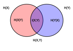
The violet is the mutual information $I(X;Y)$ .

得到随机变量 $X$ 和 $Y$ 的MI公式：

\begin{matrix} (1) & I (X; Y) = H (X) - H (X | Y) = H (Y) - H (Y | X) \end{matrix}

$I(X;Y) = H(X)-H(X \vert Y)=H(Y)-H(Y\vert X) \tag{1}$

由公式看出, $I(X;Y)$ 是当Y被观测到(observed)的条件下(即知道了 $Y$ 的熵 $H(Y)$ ),随机变量 $X$ 不确定性的归约,即Y被观测到(observed)的条件下， $I(X;Y)$ 越大， $X$ 的不确定性越小，如果随机变量 $X$ 和 $Y$ 被一一对应的映射联系在一起，那 $X$ 等于被观测 $Y$ 所确定了， $I(X;Y)$ 达到最大。

互信息最大对 $I(c;G(z,c))$ 来说，就是生成网络 $G$ 在利用 $c$ 的信息编码时，隐编码 $c$ 的损失越低越好，意思就是 $G(z,c)$ 的编码过程能够确保 $c$ 的信息被保留得越多越好。
使互信息 $I(c;G(z,c))$ 最大，即对给定任意 $x\sim P_G(x)$ ，希望 $H(P_G(c\vert x))$ 越小越好。

公式

GANs公式：

$\begin{matrix} (2) & min_{G} max_{D} V (D, G) = E_{x \sim P_{d a t a} (x)} [\log D (x)] + E_{z \sim P_{z} (z)} [\log (1 - D (G (z)))] \end{matrix}$

注：
- 在最大化D的时候，如果等式V右边第二项判断G错误，即伪造数据判断为真实数据，公式结果趋于负无穷；同理等式V右边第一项判断错误也使得最后结果趋于负无穷，所以需要最大化D，从而修改D的参数使得判别器更精确。如果判断正确，则公式V达到最大,即为0。
- 在最小化G的时候，只与等式V右边第二项有关。如果等式V右边第二项判断G错误，即伪造数据判断为真实数据，公式结果趋于负无穷；所以为了使得G伪造的数据尽可能使得D判断出错，需要最小化右侧公式第二项，使得G的参数得到调整。
InfoGANs公式：

$\begin{matrix} (3) & min_{G} max_{D} V_{I} (D, G) = V (D, G) - λ I (c; G (z, c)) \end{matrix}$ $\min_G\max_DV_I(D,G)= V(D,G)-\lambda I(c;G(z,c)) \tag{3}$
互信息损失：

$\begin{aligned} (4) & I (c; G (z, c)) & = H (c) - H (c | G (z, c)) \\ (5) & = E_{x \sim G (z, c)} [E_{c^{^{'}} \sim P (c | x)} [\log P (c^{^{'}} | x)]] + H (c) \\ (6) & = E_{x \sim G (z, c)} [D_{K L} (P (\cdot | x) ‖ Q (\cdot | x)) + E_{c^{^{'}} \sim P (c | x)} [\log Q (c^{^{'}} | x)]] + H (c) \\ (4) & \geq E_{x \sim G (z, c)} [E_{c^{^{'}} \sim P (c | x)} [\log Q (c^{^{'}} | x)]] + H (c) \end{aligned}$
- 互信息的下界是：
  $\begin{matrix} (5) & I (c; G (z, c)) = E_{x \sim P (c), x \sim G (z, c)} [\log Q ((c | x))] + H (c) \end{matrix}$ $I(c;G(z,c))=\Bbb E_{x\sim P(c),x\sim G(z,c)}\left[\log Q((c \vert x))\right] + H(c) \tag{5}$
  这里的 $H(c)$ 是先验 $P(c)$ 的熵(entropy)， $G(z,c)$ 是生成网络，因为计算后验分布 $P(c\vert x)$ 是很困难的，用 $Q(c\vert X)$ (神经网络用图片作为输入产生条件 $c$ 的分布)这样一个variational distribution对后验分布 $P(c \vert X)$ 建模。

训练

公式(3)给出了，训练的过程于原始GAN相比较，在于求出互信息(5)，即
- 采样 $c \sim P(c)$ ,
- 用 $c$ 采样 $x \sim G(z,c)$ ,
- 然后把 $c$ 和 $x$ 传给 $Q(c\vert x)$ ,
- 根据(5)最大化互信息，即后向传播修正 $G$ 和 $Q$ 网络的参数。

代码

import tensorflow as tf
from tensorflow.examples.tutorials.mnist import input_data
import numpy as np
import matplotlib.pyplot as plt
import matplotlib.gridspec as gridspec
import os


def xavier_init(size):
    in_dim = size[0]
    xavier_stddev = 1. / tf.sqrt(in_dim / 2.)
    return tf.random_normal(shape=size, stddev=xavier_stddev)


X = tf.placeholder(tf.float32, shape=[None, 784])

D_W1 = tf.Variable(xavier_init([784, 128]))
D_b1 = tf.Variable(tf.zeros(shape=[128]))

D_W2 = tf.Variable(xavier_init([128, 1]))
D_b2 = tf.Variable(tf.zeros(shape=[1]))

theta_D = [D_W1, D_W2, D_b1, D_b2]


Z = tf.placeholder(tf.float32, shape=[None, 16])
c = tf.placeholder(tf.float32, shape=[None, 10])

G_W1 = tf.Variable(xavier_init([26, 256]))
G_b1 = tf.Variable(tf.zeros(shape=[256]))

G_W2 = tf.Variable(xavier_init([256, 784]))
G_b2 = tf.Variable(tf.zeros(shape=[784]))

theta_G = [G_W1, G_W2, G_b1, G_b2]

#额外的网络Q用来近似后验分布P(c|x)
Q_W1 = tf.Variable(xavier_init([784, 128]))
Q_b1 = tf.Variable(tf.zeros(shape=[128]))

Q_W2 = tf.Variable(xavier_init([128, 10]))
Q_b2 = tf.Variable(tf.zeros(shape=[10]))

theta_Q = [Q_W1, Q_W2, Q_b1, Q_b2]

#采样噪声
def sample_Z(m, n):
    return np.random.uniform(-1., 1., size=[m, n])

#采样先验分布P(c)
def sample_c(m):
    return np.random.multinomial(1, 10*[0.1], size=m)


def generator(z, c):
    #拼接噪声分布和先验分布的数据
    inputs = tf.concat(axis=1, values=[z, c])
    G_h1 = tf.nn.relu(tf.matmul(inputs, G_W1) + G_b1)
    G_log_prob = tf.matmul(G_h1, G_W2) + G_b2
    G_prob = tf.nn.sigmoid(G_log_prob)

    return G_prob


def discriminator(x):
    D_h1 = tf.nn.relu(tf.matmul(x, D_W1) + D_b1)
    D_logit = tf.matmul(D_h1, D_W2) + D_b2
    D_prob = tf.nn.sigmoid(D_logit)

    return D_prob


def Q(x):
    Q_h1 = tf.nn.relu(tf.matmul(x, Q_W1) + Q_b1)
    Q_prob = tf.nn.softmax(tf.matmul(Q_h1, Q_W2) + Q_b2)

    return Q_prob


def plot(samples):
    fig = plt.figure(figsize=(4, 4))
    gs = gridspec.GridSpec(4, 4)
    gs.update(wspace=0.05, hspace=0.05)

    for i, sample in enumerate(samples):
        ax = plt.subplot(gs[i])
        plt.axis('off')
        ax.set_xticklabels([])
        ax.set_yticklabels([])
        ax.set_aspect('equal')
        plt.imshow(sample.reshape(28, 28), cmap='Greys_r')

    return fig


G_sample = generator(Z, c)
D_real = discriminator(X)
D_fake = discriminator(G_sample)
Q_c_given_x = Q(G_sample)

D_loss = -tf.reduce_mean(tf.log(D_real + 1e-8) + tf.log(1 - D_fake + 1e-8))
G_loss = -tf.reduce_mean(tf.log(D_fake + 1e-8))

cross_ent = tf.reduce_mean(-tf.reduce_sum(tf.log(Q_c_given_x + 1e-8) * c, 1))
ent = tf.reduce_mean(-tf.reduce_sum(tf.log(c + 1e-8) * c, 1))
Q_loss = cross_ent + ent

D_solver = tf.train.AdamOptimizer().minimize(D_loss, var_list=theta_D)
G_solver = tf.train.AdamOptimizer().minimize(G_loss, var_list=theta_G)
Q_solver = tf.train.AdamOptimizer().minimize(Q_loss, var_list=theta_G + theta_Q)

mb_size = 32
Z_dim = 16

mnist = input_data.read_data_sets('../../MNIST_data', one_hot=True)

sess = tf.Session()
sess.run(tf.global_variables_initializer())

if not os.path.exists('out/'):
    os.makedirs('out/')

i = 0

for it in range(1000000):
    if it % 1000 == 0:
        Z_noise = sample_Z(16, Z_dim)

        idx = np.random.randint(0, 10)
        c_noise = np.zeros([16, 10])
        #等于c_noise[:,idx] = 1
        c_noise[range(16), idx] = 1

        samples = sess.run(G_sample,
                           feed_dict={Z: Z_noise, c: c_noise})

        fig = plot(samples)
        plt.savefig('out/{}.png'.format(str(i).zfill(3)), bbox_inches='tight')
        i += 1
        plt.close(fig)

    X_mb, _ = mnist.train.next_batch(mb_size)
    Z_noise = sample_Z(mb_size, Z_dim)
    c_noise = sample_c(mb_size)

    _, D_loss_curr = sess.run([D_solver, D_loss],
                              feed_dict={X: X_mb, Z: Z_noise, c: c_noise})

    _, G_loss_curr = sess.run([G_solver, G_loss],
                              feed_dict={Z: Z_noise, c: c_noise})

    sess.run([Q_solver], feed_dict={Z: Z_noise, c: c_noise})

    if it % 1000 == 0:
        print('Iter: {}'.format(it))
        print('D loss: {:.4}'. format(D_loss_curr))
        print('G_loss: {:.4}'.format(G_loss_curr))
        print()

训练完成后的 $c$ 良好的编码了标签信息，如果传递c = [0, 0, 1, 0, 0, 0, 0, 0, 0, 0],会得到：

注意，并不保证结果对应到 $c$ 的顺序上。

结论

InfoGANs把prior $P(c)$ 与 noise prior $P(z)$ 映入数据分布 $P(X\vert z,c)$ 中，通过training GAN时，最大化 $c$ 与 $X$ 的互信息。这有很好的解释性，比如为什么 $X\sim P(X \vert z,c=c_i)$ 是同一类数字的图片。

启发

信息论

公式

训练

代码

结论

猜你喜欢