对于最原始的稀疏表示问题,其拉格朗日形式可写为:
s
^
=
arg
min
s
∥
y
−
A
s
∥
2
2
+
λ
∥
s
∥
0
\begin{aligned} \hat{\mathbf s} =\underset{\mathbf s}{\arg\min} \Big\Vert \mathbf y - \mathbf A \mathbf s \Big \Vert_2^2 +\lambda \Vert \mathbf s\Vert_0 \end{aligned}
s ^ = s arg min ∥ ∥ ∥ y − A s ∥ ∥ ∥ 2 2 + λ ∥ s ∥ 0
可以看出,如果将
∥
y
−
A
s
∥
2
2
\Big\Vert \mathbf y - \mathbf A \mathbf s \Big \Vert_2^2
∥ ∥ ∥ y − A s ∥ ∥ ∥ 2 2
s
\mathbf s
s 负高斯对数似然函数 ,而将
λ
∥
s
∥
0
\lambda \Vert \mathbf s\Vert_0
λ ∥ s ∥ 0
s
\mathbf s
s 先验分布的负对数 ,那么上面的优化问题实际上可解释为一个贝叶斯过程。进一步分析,求最稀疏解的问题就是一个最大后验概率(MAP:Maximum a Posteriori)估计问题。
以上分析可得出两个结论:
常见的稀疏优化问题均可以利用贝叶斯参数估计来统一表示
不同的先验概率假设会产生不同的约束效果
因此合理的先验假设是贝叶斯学习有效进行的关键。
常用的贝叶斯先验假设方法有以下几种:
贝叶斯
L
p
\mathcal L_p
L p
在基于高斯先验的稀疏表示模型中,假设要估计的稀疏向量
s
\mathbf s
s
N
(
0
,
σ
n
2
)
\mathcal N(0, \sigma_n^2)
N ( 0 , σ n 2 )
σ
n
2
\sigma_n^2
σ n 2
p
(
σ
n
2
)
∝
1
/
σ
n
2
p(\sigma_n^2) \propto 1/\sigma_n^2
p ( σ n 2 ) ∝ 1 / σ n 2
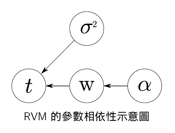
相关向量机 RVM 是一种与 SVM 类似的稀疏概率模型,其实质是一种新的贝叶斯框架下的监督学习方法。RVM 是通过多次计算参数相关性,移除不相关的基原子,从而逼近稀疏解。首先假设待估计向量中的任意一个元素都满足 Gaussian 先验分布,同时先验分布中的参数服从一个 Gamma 分布,然后计算 Gamma 分布中超参数的边缘分布,利用最大化后验概率(MAP)迭代求解出未知参数向量的均值与方差,并且利用均值进一步估计参数。该方法避免了 Laplace 先验产生的计算难度,而且可以获得信号和噪声的准确估计。
在贝叶斯学习的稀疏重构算法研究中,当前有两大热点:
相关向量机的监督学习方法
非参数贝塔过程的稀疏建模表示
稀疏贝叶斯学习(SBL)是一个强大的贝叶斯变量选择方法论,特别是当有用的变量数量很少时,优势极为突出。研究人员将 SBL 引入到稀疏信号恢复领域,作为稀疏线性回归模型中基选择的方法。
给定
t
=
y
+
z
=
Φ
w
+
z
\mathbf t = \mathbf y+\mathbf z=\mathbf \Phi \mathbf w +\mathbf z
t = y + z = Φ w + z
扫描二维码关注公众号,回复:
11236058 查看本文章
其中
z
=
[
z
1
,
⋯
 
,
z
N
]
T
\mathbf z=[z_1,\cdots, z_N]^{\rm T}
z = [ z 1 , ⋯ , z N ] T
p
(
z
)
=
∏
n
=
1
N
N
(
z
n
∣
0
,
σ
2
)
p(\mathbf z)=\prod_{n=1}^{N} \mathcal N(z_n\vert 0, \sigma^2)
p ( z ) = ∏ n = 1 N N ( z n ∣ 0 , σ 2 )
y
=
∑
m
=
1
M
w
m
ϕ
m
=
Φ
w
\mathbf y=\sum_{m=1}^{M}w_m \boldsymbol\phi_m =\mathbf \Phi \mathbf w
y = ∑ m = 1 M w m ϕ m = Φ w
w
=
[
w
1
,
⋯
 
,
w
M
]
T
\mathbf w =[w_1,\cdots, w_M]^{\rm T}
w = [ w 1 , ⋯ , w M ] T
Φ
=
[
ϕ
1
,
⋯
 
,
ϕ
M
]
\mathbf \Phi =[\boldsymbol\phi_1,\cdots, \boldsymbol\phi_M]
Φ = [ ϕ 1 , ⋯ , ϕ M ]
N
×
M
N \times M
N × M
ϕ
M
\boldsymbol\phi_M
ϕ M
M
M
M
在这里,一般
Φ
\mathbf \Phi
Φ
Φ
=
[
1
K
(
x
1
,
x
1
)
K
(
x
1
,
x
2
)
⋯
K
(
x
1
,
x
M
)
1
K
(
x
2
,
x
1
)
K
(
x
2
,
x
2
)
⋯
K
(
x
2
,
x
M
)
⋮
⋮
⋮
⋱
⋮
1
K
(
x
N
,
x
1
)
K
(
x
N
,
x
2
)
⋯
K
(
x
N
,
x
M
)
]
\mathbf \Phi= \begin{bmatrix} 1&K(\mathbf x_1,\mathbf x_1)&K(\mathbf x_1,\mathbf x_2)& \cdots &K(\mathbf x_1,\mathbf x_M)\\ 1&K(\mathbf x_2,\mathbf x_1)&K(\mathbf x_2,\mathbf x_2)& \cdots& K(\mathbf x_2,\mathbf x_M)\\ \vdots & \vdots & \vdots & \ddots & \vdots \\ 1&K(\mathbf x_N,\mathbf x_1)&K(\mathbf x_N,\mathbf x_2)& \cdots &K(\mathbf x_N,\mathbf x_M)\\ \end{bmatrix}
Φ = ⎣ ⎢ ⎢ ⎢ ⎡ 1 1 ⋮ 1 K ( x 1 , x 1 ) K ( x 2 , x 1 ) ⋮ K ( x N , x 1 ) K ( x 1 , x 2 ) K ( x 2 , x 2 ) ⋮ K ( x N , x 2 ) ⋯ ⋯ ⋱ ⋯ K ( x 1 , x M ) K ( x 2 , x M ) ⋮ K ( x N , x M ) ⎦ ⎥ ⎥ ⎥ ⎤
Φ
=
[
ϕ
(
x
1
)
,
⋯
 
,
ϕ
(
x
N
)
]
T
\mathbf \Phi =[\boldsymbol\phi(\mathbf x_1),\cdots, \boldsymbol\phi(\mathbf x_N)]^{\rm T}
Φ = [ ϕ ( x 1 ) , ⋯ , ϕ ( x N ) ] T
ϕ
(
x
i
)
=
[
1
K
(
x
i
,
x
1
)
K
(
x
i
,
x
2
)
⋮
K
(
x
i
,
x
M
)
]
\boldsymbol\phi(\mathbf x_i) = \begin{bmatrix} 1 \\ K(\mathbf x_i,\mathbf x_1) \\ K(\mathbf x_i,\mathbf x_2) \\ \vdots \\ K(\mathbf x_i,\mathbf x_M) \end{bmatrix}
ϕ ( x i ) = ⎣ ⎢ ⎢ ⎢ ⎢ ⎢ ⎡ 1 K ( x i , x 1 ) K ( x i , x 2 ) ⋮ K ( x i , x M ) ⎦ ⎥ ⎥ ⎥ ⎥ ⎥ ⎤
于是引入针对目标向量
t
\mathbf t
t
p
(
t
∣
w
,
σ
2
)
=
(
2
π
σ
2
)
−
N
2
exp
(
−
∥
t
−
Φ
w
∥
2
2
σ
2
)
p(\mathbf t \vert \mathbf w, \sigma^2) =(2\pi \sigma^2)^{-\frac{N}{2}} \exp \left( -\frac{\Vert \mathbf t - \mathbf \Phi \mathbf w \Vert^2}{2 \sigma^2} \right)
p ( t ∣ w , σ 2 ) = ( 2 π σ 2 ) − 2 N exp ( − 2 σ 2 ∥ t − Φ w ∥ 2 )
式中权值
w
\mathbf w
w
σ
2
\sigma^2
σ 2 后验密度 函数。如何应用贝叶斯估计理论,得到
w
\mathbf w
w
σ
2
\sigma^2
σ 2 使后验概率最大化来求解相关向量的加权值 。
如果采用常见的最大似然法(ML)求解待估计的
w
\mathbf w
w
σ
2
\sigma^2
σ 2 过学习 现象,因此在 RVM 框架中,我们给
w
\mathbf w
w
w
\mathbf w
w
α
i
−
1
\alpha_i^{-1}
α i − 1
p
(
w
∣
α
)
=
(
2
π
)
−
M
2
∏
m
=
1
M
α
m
1
/
2
exp
(
−
α
m
w
m
2
2
)
=
∏
i
=
1
M
N
(
w
i
∣
0
,
α
i
−
1
)
=
(
2
π
)
−
M
2
∣
Λ
α
∣
−
1
2
exp
(
−
1
2
w
T
Λ
α
−
1
w
)
\begin{aligned} p(\mathbf w \vert \boldsymbol\alpha) &=(2\pi)^{-\frac{M}{2}} \prod_{m=1}^{M} \alpha_m^{1/2} \exp \left( -\frac{\alpha_m w_m^2 }{2} \right) \\ &= \prod_{i=1}^{M} \mathcal N(w_i \vert 0, \alpha_i^{-1}) \\ &=(2\pi)^{\frac{-M}{2}} \Big\vert \mathbf{\Lambda}_{\alpha} \Big\vert^{-\frac{1}{2}} \exp\left({-\frac{1}{2}\mathbf{ w}^{\rm T}\mathbf{\Lambda_{\alpha}^{-1}\mathbf{ w}}} \right) \end{aligned}
p ( w ∣ α ) = ( 2 π ) − 2 M m = 1 ∏ M α m 1 / 2 exp ( − 2 α m w m 2 ) = i = 1 ∏ M N ( w i ∣ 0 , α i − 1 ) = ( 2 π ) 2 − M ∣ ∣ ∣ Λ α ∣ ∣ ∣ − 2 1 exp ( − 2 1 w T Λ α − 1 w )
Λ
α
=
diag
(
[
α
1
−
1
,
⋯
 
,
α
M
−
1
]
)
\mathbf{\Lambda}_{\alpha}=\text{diag}([\alpha_1^{-1},\cdots,\alpha_M^{-1}])
Λ α = diag ( [ α 1 − 1 , ⋯ , α M − 1 ] )
其次再对
α
\boldsymbol \alpha
α
p
(
α
)
=
∏
i
=
1
M
Γ
(
α
i
∣
a
,
b
)
=
p
(
α
∣
a
,
b
)
p(\boldsymbol\alpha) = \prod_{i=1}^{M} \Gamma(\alpha_i \vert a,b) = p(\boldsymbol\alpha \vert a,b)
p ( α ) = i = 1 ∏ M Γ ( α i ∣ a , b ) = p ( α ∣ a , b )
Γ
(
x
∣
a
,
b
)
=
b
a
x
a
−
1
e
−
b
x
f
Γ
(
a
)
\Gamma(x \vert a,b) = \frac{ b^a x^{a-1}e^{-bx}}{f_{\Gamma}(a)}
Γ ( x ∣ a , b ) = f Γ ( a ) b a x a − 1 e − b x https://blog.csdn.net/chenshulong/article/details/79027103 。
f
Γ
(
x
)
=
∫
0
∞
t
x
−
1
e
−
t
d
t
f_{\Gamma}(x) =\int_0^{\infty}t^{x-1}e^{-t} \text{d}t
f Γ ( x ) = ∫ 0 ∞ t x − 1 e − t d t
f
Γ
(
x
+
1
)
=
x
f
Γ
(
x
)
f_{\Gamma}(x+1) =x f_{\Gamma}(x)
f Γ ( x + 1 ) = x f Γ ( x )
f
Γ
(
n
)
=
(
n
−
1
)
!
f_{\Gamma}(n) = (n-1)!
f Γ ( n ) = ( n − 1 ) !
结合
p
(
w
∣
α
)
p(\mathbf w \vert \boldsymbol\alpha)
p ( w ∣ α )
p
(
α
∣
a
,
b
)
p(\boldsymbol\alpha \vert a,b)
p ( α ∣ a , b )
p
(
w
∣
a
,
b
)
=
∏
i
=
1
M
∫
0
∞
N
(
w
i
∣
0
,
α
i
−
1
)
Γ
(
α
i
∣
a
,
b
)
d
α
i
p(\mathbf w \vert a,b)= \prod_{i=1}^{M} \int_{0}^{\infty} \mathcal N(w_i \vert 0, \alpha_i^{-1}) \Gamma(\alpha_i \vert a,b) \text{d}\alpha_i
p ( w ∣ a , b ) = i = 1 ∏ M ∫ 0 ∞ N ( w i ∣ 0 , α i − 1 ) Γ ( α i ∣ a , b ) d α i
α
\boldsymbol\alpha
α
w
\mathbf w
w
α
i
\alpha_i
α i
α
i
\alpha_i
α i
w
i
w_i
w i
p
(
w
i
)
=
N
(
0
,
α
i
−
1
)
p(w_i)=\mathcal{N}(0,\alpha_i^{-1})
p ( w i ) = N ( 0 , α i − 1 )
α
i
\alpha_i
α i
p
(
w
i
)
p(w_i)
p ( w i )
w
i
=
0
w_i=0
w i = 0
下面详细介绍基于 RVM 机制的快速贝叶斯学习算法(FSBL)。根据贝叶斯稀疏重构理论 , 可以通过统计概率方法解决,即:
w
^
=
arg
max
w
[
p
(
w
^
,
σ
2
,
α
∣
t
)
]
\hat{\mathbf w} =\underset{{\mathbf w} }{\arg\max} \Big[ p( \hat{\mathbf w}, \sigma^2, \boldsymbol \alpha\vert \mathbf t) \Big]
w ^ = w arg max [ p ( w ^ , σ 2 , α ∣ t ) ]
α
\boldsymbol \alpha
α
p
(
w
^
,
σ
2
,
α
∣
t
)
=
p
(
w
^
∣
σ
2
,
α
,
t
)
p
(
σ
2
,
α
∣
t
)
\boxed{ \textcolor{blue}{ p( \hat{\mathbf w}, \sigma^2, \boldsymbol \alpha\vert \mathbf t) = p( \hat{\mathbf w} \vert \sigma^2, \boldsymbol \alpha,\mathbf t) p( \sigma^2, \boldsymbol \alpha \vert \mathbf t) } }
p ( w ^ , σ 2 , α ∣ t ) = p ( w ^ ∣ σ 2 , α , t ) p ( σ 2 , α ∣ t )
接下来我们主要围绕上面这个公式展开推导
首先从公式的第一项
p
(
w
^
∣
σ
2
,
α
,
t
)
p( \hat{\mathbf w} \vert \sigma^2, \boldsymbol \alpha,\mathbf t)
p ( w ^ ∣ σ 2 , α , t )
然后分析第二项
p
(
σ
2
,
α
∣
t
)
p( \sigma^2, \boldsymbol \alpha \vert \mathbf t)
p ( σ 2 , α ∣ t )
根据上面示意图中的概率依赖关系,其中
p
(
w
^
∣
σ
2
,
α
,
t
)
=
p
(
w
,
t
∣
σ
2
,
α
)
p
(
t
∣
σ
2
,
α
)
=
p
(
w
∣
α
)
p
(
t
∣
w
,
σ
2
)
p
(
t
∣
σ
2
,
α
)
=
p
(
w
∣
α
)
p
(
t
∣
w
,
σ
2
)
∫
p
(
w
∣
α
)
p
(
t
∣
w
,
σ
2
)
d
w
=
(
2
π
)
−
M
2
∣
Σ
∣
−
1
/
2
exp
{
−
1
2
(
w
−
μ
)
T
Σ
−
1
(
w
−
μ
)
}
\begin{aligned} p( \hat{\mathbf w} \vert \sigma^2, \boldsymbol \alpha,\mathbf t) &= \frac{p( {\mathbf w},\mathbf t \vert \sigma^2, \boldsymbol \alpha) }{p( \mathbf t \vert \sigma^2, \boldsymbol \alpha)} \\ &=\frac{p(\mathbf w \vert \boldsymbol\alpha) p(\mathbf t \vert \mathbf w, \sigma^2)}{p( \mathbf t \vert \sigma^2, \boldsymbol \alpha)} \\ &=\frac{p(\mathbf w \vert \boldsymbol\alpha) p(\mathbf t \vert \mathbf w, \sigma^2)}{\int p(\mathbf w \vert \boldsymbol\alpha) p(\mathbf t \vert \mathbf w, \sigma^2) \text{d}\mathbf w} \\ &=(2\pi)^{-\frac{M}{2}} \Big\vert \mathbf \Sigma \Big\vert^{-1/2} \exp\left\{ -\frac{1}{2} (\mathbf w- \bm{\mu})^{\rm T} \mathbf \Sigma^{-1}(\mathbf w- \bm{\mu}) \right\} \end{aligned}
p ( w ^ ∣ σ 2 , α , t ) = p ( t ∣ σ 2 , α ) p ( w , t ∣ σ 2 , α ) = p ( t ∣ σ 2 , α ) p ( w ∣ α ) p ( t ∣ w , σ 2 ) = ∫ p ( w ∣ α ) p ( t ∣ w , σ 2 ) d w p ( w ∣ α ) p ( t ∣ w , σ 2 ) = ( 2 π ) − 2 M ∣ ∣ ∣ Σ ∣ ∣ ∣ − 1 / 2 exp { − 2 1 ( w − μ ) T Σ − 1 ( w − μ ) }
推导过程如下:
p
(
t
∣
σ
2
,
α
)
=
∫
(
2
π
σ
2
)
−
N
/
2
(
2
π
)
−
M
/
2
∣
Λ
α
∣
−
1
2
exp
[
−
1
2
σ
2
(
t
−
Φ
w
)
T
(
t
−
Φ
w
)
−
1
2
w
T
Λ
α
−
1
w
]
d
w
\begin{aligned} p( \mathbf t \vert \sigma^2, \boldsymbol \alpha)=\int (2\pi\sigma^2)^{-N/2}(2\pi)^{-M/2} \Big|\mathbf{\Lambda}_{\alpha}\Big|^{-\frac{1}{2}} \exp\bigg[-\frac{1}{2\sigma^2}(\mathbf{t}-\mathbf{\Phi w})^{\rm T}(\mathbf{t}-\mathbf{\Phi w})-\frac{1}{2}\mathbf {w}^{\rm T} \mathbf{\Lambda_{\alpha}^{-1} w} \bigg] \text{d}\mathbf w \end{aligned}
p ( t ∣ σ 2 , α ) = ∫ ( 2 π σ 2 ) − N / 2 ( 2 π ) − M / 2 ∣ ∣ ∣ Λ α ∣ ∣ ∣ − 2 1 exp [ − 2 σ 2 1 ( t − Φ w ) T ( t − Φ w ) − 2 1 w T Λ α − 1 w ] d w
其实该式可以看成两个高斯函数进行卷积 ,根据高斯函数性质知,两个高斯函数卷积的结果仍为高斯函数。所以只需要求得卷积后的高斯函数的均值和期望 ,就相当于求出上式的积分了。
取其指数,令
Q
=
−
1
2
σ
2
(
t
−
Φ
w
)
T
(
t
−
Φ
w
)
−
1
2
w
T
Λ
α
−
1
w
=
−
1
2
σ
2
(
t
T
t
−
t
T
Φ
w
−
w
T
Φ
T
t
)
−
1
2
σ
2
w
T
Φ
T
Φ
w
−
1
2
w
T
Λ
α
−
1
w
=
−
1
2
σ
2
[
w
T
(
Φ
T
Φ
+
σ
2
Λ
α
−
1
)
w
−
t
T
Φ
w
−
w
T
Φ
T
t
+
t
T
t
]
\begin{aligned} Q &=-\frac{1}{2\sigma^2}(\mathbf{t}-\mathbf{\Phi w})^{\rm T}(\mathbf{t}-\mathbf{\Phi w})-\frac{1}{2}\mathbf {w}^{\rm T} \mathbf{\Lambda_{\alpha}^{-1} w} \\ &=-\frac{1}{2\sigma^2} \bigg(\mathbf t^{\rm T}\mathbf t -\mathbf t^{\rm T}\mathbf{ \Phi w}-\mathbf w^{\rm T}\mathbf{\Phi}^{\rm T}\mathbf t \bigg) -\frac{1}{2\sigma^2}\mathbf w^{\rm T}\mathbf{\Phi}^{\rm T}\mathbf{ \Phi w}-\frac{1}{2}\mathbf {w}^{\rm T} \mathbf{\Lambda_{\alpha}^{-1} w} \\ &=-\frac{1}{2\sigma^2} \bigg[ \mathbf{w}^{\rm T}(\mathbf{\Phi}^{\rm T}\mathbf{\Phi}+\sigma^2\mathbf{\Lambda}_{\alpha}^{-1})\mathbf{w}-\mathbf{t}^{\rm T}\mathbf{\Phi}\mathbf{w}-\mathbf{w}^{\rm T}\mathbf{\Phi}^{\rm T}\mathbf{t}+\mathbf{t}^{\rm T}\mathbf{t} \bigg] \end{aligned}
Q = − 2 σ 2 1 ( t − Φ w ) T ( t − Φ w ) − 2 1 w T Λ α − 1 w = − 2 σ 2 1 ( t T t − t T Φ w − w T Φ T t ) − 2 σ 2 1 w T Φ T Φ w − 2 1 w T Λ α − 1 w = − 2 σ 2 1 [ w T ( Φ T Φ + σ 2 Λ α − 1 ) w − t T Φ w − w T Φ T t + t T t ]
p
(
t
∣
σ
2
,
α
)
=
(
2
π
σ
2
)
−
N
/
2
(
2
π
)
−
M
/
2
∣
Λ
α
∣
−
1
2
∫
exp
(
Q
(
w
)
)
d
w
p( \mathbf t \vert \sigma^2, \boldsymbol \alpha)= (2\pi\sigma^2)^{-N/2}(2\pi)^{-M/2} \Big|\mathbf{\Lambda}_{\alpha}\Big|^{-\frac{1}{2}} \int \exp\bigg(Q(\mathbf w)\bigg)\text{d}\mathbf w
p ( t ∣ σ 2 , α ) = ( 2 π σ 2 ) − N / 2 ( 2 π ) − M / 2 ∣ ∣ ∣ Λ α ∣ ∣ ∣ − 2 1 ∫ exp ( Q ( w ) ) d w
Q
Q
Q
w
\mathbf w
w
∫
ω
exp
[
−
(
A
ω
+
b
)
2
]
d
ω
=
C
\int_{\bm{\omega}}\exp\left[{-(\bm{A\omega}+\bm{b})^2} \right] \text{d}\bm{\omega}=C
∫ ω exp [ − ( A ω + b ) 2 ] d ω = C
C
C
C
Q
Q
Q
−
(
A
w
+
b
)
2
+
f
(
t
,
σ
2
)
-(\mathbf{A w}+\mathbf{b})^2+f(\mathbf t, \sigma^2)
− ( A w + b ) 2 + f ( t , σ 2 )
f
(
t
,
σ
2
)
f(t,σ2)
f ( t , σ 2 )
A
w
+
b
=
0
\mathbf{A w}+\mathbf{b}=0
A w + b = 0
w
\mathbf{w}
w
f
(
t
,
σ
2
)
f(\mathbf t, \sigma^2)
f ( t , σ 2 )
w
\mathbf{w}
w
d
Q
d
w
=
−
1
σ
2
[
(
Φ
T
Φ
+
σ
2
Λ
α
−
1
)
w
−
Φ
T
t
]
=
0
w
∗
=
(
Φ
T
Φ
+
σ
2
Λ
α
−
1
)
†
Φ
T
t
\begin{aligned} \frac{dQ}{d\bf{w}}&=-\frac{1}{\sigma^2} \bigg[ (\mathbf{\Phi}^{\rm T}\mathbf{\Phi}+\sigma^2\mathbf{\Lambda}_{\alpha}^{-1})\mathbf{w}-\mathbf{\Phi}^{\rm T}\mathbf{t} \bigg]=0 \\ \mathbf w^* &=(\mathbf{\Phi}^{\rm T}\mathbf{\Phi}+\sigma^2\mathbf{\Lambda}_{\alpha}^{-1})^{\dagger} \mathbf{\Phi}^{\rm T}\mathbf{t} \end{aligned}
d w d Q w ∗ = − σ 2 1 [ ( Φ T Φ + σ 2 Λ α − 1 ) w − Φ T t ] = 0 = ( Φ T Φ + σ 2 Λ α − 1 ) † Φ T t
由于
d
Q
d
w
=
0
⟺
A
w
+
b
=
0
\frac{dQ}{d\bf{w}}=0 \Longleftrightarrow \mathbf{A w}+\mathbf{b}=0
d w d Q = 0 ⟺ A w + b = 0
Φ
T
Φ
+
σ
2
Λ
α
−
1
=
B
\mathbf{\Phi}^{\rm T}\mathbf{\Phi}+\sigma^2\mathbf{\Lambda}_{\alpha}^{-1}=\mathbf B
Φ T Φ + σ 2 Λ α − 1 = B
w
∗
=
B
†
Φ
T
t
\mathbf w^* =\mathbf B^{\dagger} \mathbf{\Phi}^{\rm T}\mathbf{t}
w ∗ = B † Φ T t
Q
(
w
)
Q(\mathbf w)
Q ( w )
Q
(
w
∗
)
=
−
1
2
σ
2
[
w
T
B
w
−
t
T
Φ
w
−
w
T
Φ
T
t
+
t
T
t
]
=
−
1
2
σ
2
[
t
T
(
I
−
Φ
B
†
Φ
T
)
t
]
=
f
(
t
,
σ
2
)
p
(
t
∣
σ
2
,
α
)
=
(
2
π
σ
2
)
−
N
/
2
(
2
π
)
−
M
/
2
∣
Λ
α
∣
−
1
2
∫
exp
(
Q
(
w
)
)
d
w
=
(
2
π
σ
2
)
−
N
/
2
(
2
π
)
−
M
/
2
∣
Λ
α
∣
−
1
2
C
⋅
exp
(
−
1
2
σ
2
[
t
T
(
I
−
Φ
B
†
Φ
T
)
t
]
)
\begin{aligned} Q(\mathbf w^*)&=-\frac{1}{2\sigma^2} \bigg[ \mathbf{w}^{\rm T}\mathbf B\mathbf{w}-\mathbf{t}^{\rm T}\mathbf{\Phi}\mathbf{w}-\mathbf{w}^{\rm T}\mathbf{\Phi}^{\rm T}\mathbf{t}+\mathbf{t}^{\rm T}\mathbf{t} \bigg] \\ &=-\frac{1}{2\sigma^2} \bigg[ \mathbf{t}^{\rm T} \left( \mathbf{I}-\mathbf{\Phi}\mathbf B^{\dagger}\mathbf{\Phi}^{\rm T} \right) \mathbf{t} \bigg] = f(\mathbf t, \sigma^2) \\ p( \mathbf t \vert \sigma^2, \boldsymbol \alpha)&= (2\pi\sigma^2)^{-N/2}(2\pi)^{-M/2} \Big|\mathbf{\Lambda}_{\alpha}\Big|^{-\frac{1}{2}} \int \exp\bigg(Q(\mathbf w)\bigg)\text{d}\mathbf w \\ &=(2\pi\sigma^2)^{-N/2}(2\pi)^{-M/2} \Big|\mathbf{\Lambda}_{\alpha}\Big|^{-\frac{1}{2}} C \cdot \exp\bigg( -\frac{1}{2\sigma^2} \bigg[ \mathbf{t}^{\rm T} \left( \mathbf{I}-\mathbf{\Phi}\mathbf B^{\dagger}\mathbf{\Phi}^{\rm T} \right) \mathbf{t} \bigg] \bigg) \end{aligned}
Q ( w ∗ ) p ( t ∣ σ 2 , α ) = − 2 σ 2 1 [ w T B w − t T Φ w − w T Φ T t + t T t ] = − 2 σ 2 1 [ t T ( I − Φ B † Φ T ) t ] = f ( t , σ 2 ) = ( 2 π σ 2 ) − N / 2 ( 2 π ) − M / 2 ∣ ∣ ∣ Λ α ∣ ∣ ∣ − 2 1 ∫ exp ( Q ( w ) ) d w = ( 2 π σ 2 ) − N / 2 ( 2 π ) − M / 2 ∣ ∣ ∣ Λ α ∣ ∣ ∣ − 2 1 C ⋅ exp ( − 2 σ 2 1 [ t T ( I − Φ B † Φ T ) t ] )
p
(
t
∣
σ
2
,
α
)
p( \mathbf t \vert \sigma^2, \boldsymbol \alpha)
p ( t ∣ σ 2 , α )
Σ
t
\mathbf\Sigma_t
Σ t
Σ
t
−
1
=
1
σ
2
(
I
−
Φ
B
†
Φ
T
)
\begin{aligned} \mathbf\Sigma_t^{-1}=\frac{1}{\sigma^2} \left( \mathbf{I}-\mathbf{\Phi}\mathbf B^{\dagger}\mathbf{\Phi}^{\rm T} \right) \end{aligned}
Σ t − 1 = σ 2 1 ( I − Φ B † Φ T )
Σ
t
\mathbf\Sigma_t
Σ t
Σ
t
=
σ
2
(
I
−
Φ
B
†
Φ
T
)
−
1
=
σ
2
[
I
−
Φ
(
Φ
T
Φ
+
σ
2
Λ
α
−
1
)
−
1
Φ
T
]
−
1
=
σ
2
I
+
Φ
Λ
α
Φ
T
\begin{aligned} \mathbf\Sigma_t&={\sigma^2} \big( \mathbf{I}-\mathbf{\Phi}\mathbf B^{\dagger}\mathbf{\Phi}^{\rm T} \big)^{-1} \\ &={\sigma^2} \bigg[ \mathbf{I}-\mathbf{\Phi} \big( \mathbf{\Phi}^{\rm T}\mathbf{\Phi}+\sigma^2\mathbf{\Lambda}_{\alpha}^{-1} \big)^{-1} \mathbf{\Phi}^{\rm T} \bigg]^{-1} \\ &=\sigma^2 \mathbf{I}+\mathbf{\Phi}\mathbf{\Lambda}_{\alpha}\mathbf{\Phi}^{\rm T} \end{aligned}
Σ t = σ 2 ( I − Φ B † Φ T ) − 1 = σ 2 [ I − Φ ( Φ T Φ + σ 2 Λ α − 1 ) − 1 Φ T ] − 1 = σ 2 I + Φ Λ α Φ T
这是在写博客时候第二次遇到矩阵求逆公式 参考1 参考2
(
A
+
U
B
V
)
−
1
=
A
−
1
−
A
−
1
U
B
(
I
+
V
A
−
1
U
B
)
−
1
V
A
−
1
\boxed{ \textcolor{red}{ (\mathbf A+\mathbf{UBV})^{-1}=\mathbf A^{-1}- \mathbf A^{-1}\mathbf{UB}(\mathbf I+\mathbf{VA}^{-1}\mathbf{UB})^{-1}\mathbf{VA}^{-1} } }
( A + U B V ) − 1 = A − 1 − A − 1 U B ( I + V A − 1 U B ) − 1 V A − 1
Φ
T
Φ
+
σ
2
Λ
α
−
1
=
B
\mathbf{\Phi}^{\rm T}\mathbf{\Phi}+\sigma^2\mathbf{\Lambda}_{\alpha}^{-1}=\mathbf B
Φ T Φ + σ 2 Λ α − 1 = B
[
I
−
Φ
(
Φ
T
Φ
+
σ
2
Λ
α
−
1
)
−
1
Φ
T
]
−
1
=
I
+
Φ
B
−
1
(
I
−
Φ
T
Φ
B
−
1
)
−
1
Φ
T
=
I
+
Φ
[
(
I
−
Φ
T
Φ
B
−
1
)
B
]
−
1
Φ
T
=
I
+
Φ
(
B
−
Φ
T
Φ
)
−
1
Φ
T
=
I
+
σ
−
2
Φ
Λ
α
Φ
T
\begin{aligned} &\bigg[ \mathbf{I}-\mathbf{\Phi} \big( \mathbf{\Phi}^{\rm T}\mathbf{\Phi}+\sigma^2\mathbf{\Lambda}_{\alpha}^{-1} \big)^{-1} \mathbf{\Phi}^{\rm T} \bigg]^{-1} \\ =& \ \ \mathbf{I}+\mathbf{\Phi} \textcolor{blue}{\mathbf B^{-1}\big( \mathbf{I} -\mathbf{\Phi}^{\rm T}\mathbf{\Phi}\mathbf B^{-1} \big)^{-1}} \mathbf{\Phi}^{\rm T} \\ =& \ \ \mathbf{I}+\mathbf{\Phi} \bigg[ \big( \mathbf{I} -\mathbf{\Phi}^{\rm T}\mathbf{\Phi}\mathbf B^{-1} \big) \mathbf B \bigg]^{-1} \mathbf{\Phi}^{\rm T} \\ =& \ \ \mathbf{I}+\mathbf{\Phi} \big( \mathbf{B} -\mathbf{\Phi}^{\rm T}\mathbf{\Phi} \big)^{-1} \mathbf{\Phi}^{\rm T} \\ =& \ \ \mathbf{I}+ \sigma^{-2}\mathbf{\Phi} \mathbf{\Lambda}_{\alpha} \mathbf{\Phi}^{\rm T} \end{aligned}
= = = = [ I − Φ ( Φ T Φ + σ 2 Λ α − 1 ) − 1 Φ T ] − 1 I + Φ B − 1 ( I − Φ T Φ B − 1 ) − 1 Φ T I + Φ [ ( I − Φ T Φ B − 1 ) B ] − 1 Φ T I + Φ ( B − Φ T Φ ) − 1 Φ T I + σ − 2 Φ Λ α Φ T
至此,我们对于协方差的推导到此结束。
利用前面的结果,分母部分
p
(
t
∣
σ
2
,
α
)
p( \mathbf t \vert \sigma^2, \boldsymbol \alpha)
p ( t ∣ σ 2 , α )
p
(
w
^
∣
σ
2
,
α
,
t
)
=
p
(
w
∣
α
)
p
(
t
∣
w
,
σ
2
)
p
(
t
∣
σ
2
,
α
)
\begin{aligned} p( \hat{\mathbf w} \vert \sigma^2, \boldsymbol \alpha,\mathbf t) &=\frac{p(\mathbf w \vert \boldsymbol\alpha) p(\mathbf t \vert \mathbf w, \sigma^2)}{p( \mathbf t \vert \sigma^2, \boldsymbol \alpha)} \\ \end{aligned}
p ( w ^ ∣ σ 2 , α , t ) = p ( t ∣ σ 2 , α ) p ( w ∣ α ) p ( t ∣ w , σ 2 )
p
(
w
∣
α
)
=
(
2
π
)
−
M
2
∣
Λ
α
∣
−
1
2
exp
(
−
1
2
w
T
Λ
α
−
1
w
)
p
(
t
∣
w
,
σ
2
)
=
(
2
π
σ
2
)
−
N
2
exp
(
−
1
2
σ
2
(
t
−
Φ
w
)
T
(
t
−
Φ
w
)
)
\boxed{ \begin{aligned} p(\mathbf w \vert \boldsymbol\alpha)&= (2\pi)^{\frac{-M}{2}} \Big\vert \mathbf{\Lambda}_{\alpha} \Big\vert^{-\frac{1}{2}} \exp\left({-\frac{1}{2}\mathbf{ w}^{\rm T}\mathbf{\Lambda_{\alpha}^{-1}\mathbf{ w}}} \right) \\ p(\mathbf t \vert \mathbf w, \sigma^2) &=(2\pi \sigma^2)^{-\frac{N}{2}} \exp \left(-\frac{1}{2\sigma^2}(\mathbf{t}-\mathbf{\Phi w})^{\rm T}(\mathbf{t}-\mathbf{\Phi w}) \right) \end{aligned} }
p ( w ∣ α ) p ( t ∣ w , σ 2 ) = ( 2 π ) 2 − M ∣ ∣ ∣ Λ α ∣ ∣ ∣ − 2 1 exp ( − 2 1 w T Λ α − 1 w ) = ( 2 π σ 2 ) − 2 N exp ( − 2 σ 2 1 ( t − Φ w ) T ( t − Φ w ) )
(
2
π
σ
2
)
−
N
2
(
2
π
)
−
M
2
∣
Λ
α
∣
−
1
2
=
C
1
(2\pi\sigma^2)^{-\frac{N}{2}}(2\pi)^{-\frac{M}{2}} \Big|\mathbf{\Lambda}_{\alpha}\Big|^{-\frac{1}{2}} =C_1
( 2 π σ 2 ) − 2 N ( 2 π ) − 2 M ∣ ∣ ∣ Λ α ∣ ∣ ∣ − 2 1 = C 1
p
(
w
∣
α
)
p
(
t
∣
w
,
σ
2
)
=
C
1
⋅
exp
(
−
1
2
σ
2
[
w
T
B
w
−
t
T
Φ
w
−
w
T
Φ
T
t
+
t
T
t
]
)
p
(
t
∣
σ
2
,
α
)
=
(
2
π
)
−
N
2
∣
Σ
t
∣
−
1
2
exp
(
−
1
2
[
t
T
(
Σ
t
)
−
1
t
]
)
\begin{aligned} p(\mathbf w \vert \boldsymbol\alpha) p(\mathbf t \vert \mathbf w, \sigma^2) &= C_1 \cdot \exp\bigg( -\frac{1}{2\sigma^2} \bigg[ \mathbf{w}^{\rm T}\mathbf B\mathbf{w}-\mathbf{t}^{\rm T}\mathbf{\Phi}\mathbf{w}-\mathbf{w}^{\rm T}\mathbf{\Phi}^{\rm T}\mathbf{t}+\mathbf{t}^{\rm T}\mathbf{t} \bigg] \bigg) \\ \textcolor{blue}{ p( \mathbf t \vert \sigma^2, \boldsymbol \alpha) } &\textcolor{blue}{=(2\pi)^{-\frac{N}{2}} \Big\vert \mathbf{\Sigma}_t \Big\vert^{-\frac{1}{2}} \exp\bigg( -\frac{1}{2} \bigg[ \mathbf{t}^{\rm T} \left( \mathbf{\Sigma}_t \right)^{-1} \mathbf{t} \bigg] \bigg) } \end{aligned}
p ( w ∣ α ) p ( t ∣ w , σ 2 ) p ( t ∣ σ 2 , α ) = C 1 ⋅ exp ( − 2 σ 2 1 [ w T B w − t T Φ w − w T Φ T t + t T t ] ) = ( 2 π ) − 2 N ∣ ∣ ∣ Σ t ∣ ∣ ∣ − 2 1 exp ( − 2 1 [ t T ( Σ t ) − 1 t ] )
p
(
w
^
∣
σ
2
,
α
,
t
)
=
C
2
exp
(
−
1
2
σ
2
[
w
T
B
w
−
t
T
Φ
w
−
w
T
Φ
T
t
+
t
T
t
]
−
1
2
t
T
Σ
t
−
1
t
)
=
C
2
exp
(
Q
w
(
w
)
)
\begin{aligned} p( \hat{\mathbf w} \vert \sigma^2, \boldsymbol \alpha,\mathbf t) &=C_2 \exp\bigg( -\frac{1}{2\sigma^2} \bigg[ \mathbf{w}^{\rm T}\mathbf B\mathbf{w}-\mathbf{t}^{\rm T}\mathbf{\Phi}\mathbf{w}-\mathbf{w}^{\rm T}\mathbf{\Phi}^{\rm T}\mathbf{t}+\mathbf{t}^{\rm T}\mathbf{t} \bigg] -\frac{1}{2}\mathbf{t}^{\rm T} \mathbf{\Sigma}_t^{-1} \mathbf{t} \bigg) \\ &=C_2 \exp\bigg( Q_w(\mathbf w)\bigg) \end{aligned}
p ( w ^ ∣ σ 2 , α , t ) = C 2 exp ( − 2 σ 2 1 [ w T B w − t T Φ w − w T Φ T t + t T t ] − 2 1 t T Σ t − 1 t ) = C 2 exp ( Q w ( w ) )
根据多维高斯函数的形式
N
(
x
∣
μ
,
Σ
)
=
(
2
π
)
−
d
/
2
∣
Σ
∣
−
1
/
2
exp
{
−
1
2
(
x
−
μ
)
T
Σ
−
1
(
x
−
μ
)
}
\mathcal N(\mathbf x \vert \bm\mu,\mathbf \Sigma)= (2\pi)^{-d/2} \Big\vert \mathbf \Sigma \Big\vert^{-1/2} \exp\bigg\{ -\frac{1}{2} (\mathbf x-\bm\mu) ^{\rm T} \mathbf \Sigma^{-1} (\mathbf x-\bm\mu) \bigg\}
N ( x ∣ μ , Σ ) = ( 2 π ) − d / 2 ∣ ∣ ∣ Σ ∣ ∣ ∣ − 1 / 2 exp { − 2 1 ( x − μ ) T Σ − 1 ( x − μ ) }
Q
1
=
−
1
2
(
x
−
μ
)
T
Σ
−
1
(
x
−
μ
)
Q_1 =-\frac{1}{2} (\mathbf x-\bm\mu) ^{\rm T} \mathbf \Sigma^{-1} (\mathbf x-\bm\mu)
Q 1 = − 2 1 ( x − μ ) T Σ − 1 ( x − μ )
d
Q
1
d
x
=
0
⟹
x
^
0
=
μ
d
2
Q
1
d
x
2
=
−
Σ
−
1
\begin{aligned} \frac{dQ_1}{d\bf{x}}&=0 \Longrightarrow \hat{\mathbf x}_0 = \bm\mu \\ \frac{d^2Q_1}{d\mathbf{x}^2}&=- \mathbf \Sigma^{-1} \end{aligned}
d x d Q 1 d x 2 d 2 Q 1 = 0 ⟹ x ^ 0 = μ = − Σ − 1
因此,可以得出
p
(
w
^
∣
σ
2
,
α
,
t
)
p( \hat{\mathbf w} \vert \sigma^2, \boldsymbol \alpha,\mathbf t)
p ( w ^ ∣ σ 2 , α , t )
μ
w
\bm\mu_w
μ w
Σ
w
\mathbf \Sigma_w
Σ w
d
Q
w
d
w
=
0
⟹
μ
w
=
B
−
1
Φ
T
t
=
(
Φ
T
Φ
+
σ
2
Λ
α
−
1
)
−
1
Φ
T
t
−
d
2
Q
w
d
w
2
=
Σ
w
−
1
=
1
σ
2
B
=
1
σ
2
(
Φ
T
Φ
+
σ
2
Λ
α
−
1
)
=
1
σ
2
Φ
T
Φ
+
Λ
α
−
1
\begin{aligned} \frac{dQ_w}{d\bf{w}}&=0 \Longrightarrow \bm\mu_w =\mathbf B^{-1} \mathbf{\Phi}^{\rm T}\mathbf t =(\mathbf{\Phi}^{\rm T}\mathbf{\Phi}+\sigma^2\mathbf{\Lambda}_{\alpha}^{-1})^{-1} \mathbf{\Phi}^{\rm T}\mathbf t \\ -\frac{d^2Q_w}{d\mathbf{w}^2}&= \mathbf \Sigma_w^{-1} = \frac{1}{\sigma^2}\mathbf B = \frac{1}{\sigma^2} (\mathbf{\Phi}^{\rm T}\mathbf{\Phi}+\sigma^2\mathbf{\Lambda}_{\alpha}^{-1}) = \frac{1}{\sigma^2}\mathbf{\Phi}^{\rm T}\mathbf{\Phi}+\mathbf{\Lambda}_{\alpha}^{-1} \end{aligned}
d w d Q w − d w 2 d 2 Q w = 0 ⟹ μ w = B − 1 Φ T t = ( Φ T Φ + σ 2 Λ α − 1 ) − 1 Φ T t = Σ w − 1 = σ 2 1 B = σ 2 1 ( Φ T Φ + σ 2 Λ α − 1 ) = σ 2 1 Φ T Φ + Λ α − 1
p
(
w
^
∣
σ
2
,
α
,
t
)
=
(
2
π
)
−
M
2
∣
Σ
w
∣
−
1
/
2
exp
{
−
1
2
(
w
−
μ
w
)
T
Σ
w
−
1
(
w
−
μ
w
)
}
\boxed{ p( \hat{\mathbf w} \vert \sigma^2, \boldsymbol \alpha,\mathbf t) = (2\pi)^{-\frac{M}{2}} \Big\vert \mathbf \Sigma_w \Big\vert^{-1/2} \exp\left\{ -\frac{1}{2} (\mathbf w- \bm{\mu}_w)^{\rm T} \mathbf \Sigma_w^{-1}(\mathbf w- \bm{\mu}_w) \right\} }
p ( w ^ ∣ σ 2 , α , t ) = ( 2 π ) − 2 M ∣ ∣ ∣ Σ w ∣ ∣ ∣ − 1 / 2 exp { − 2 1 ( w − μ w ) T Σ w − 1 ( w − μ w ) }
其中
Σ
w
−
1
=
1
σ
2
Φ
T
Φ
+
Λ
α
−
1
μ
w
=
σ
−
2
Σ
w
Φ
T
t
\boxed{ \begin{aligned} \mathbf \Sigma_w^{-1} &= \frac{1}{\sigma^2}\mathbf{\Phi}^{\rm T}\mathbf{\Phi}+\mathbf{\Lambda}_{\alpha}^{-1} \\ \bm\mu_w &= \sigma^{-2} \mathbf \Sigma_w \mathbf{\Phi}^{\rm T}\mathbf t \end{aligned} }
Σ w − 1 μ w = σ 2 1 Φ T Φ + Λ α − 1 = σ − 2 Σ w Φ T t
至此,第一项推导完毕,过程可真是长啊!
回顾前面提到的贝叶斯公式:
p
(
w
^
,
σ
2
,
α
∣
t
)
=
p
(
w
^
∣
σ
2
,
α
,
t
)
p
(
σ
2
,
α
∣
t
)
\boxed{ \textcolor{blue}{ p( \hat{\mathbf w}, \sigma^2, \boldsymbol \alpha\vert \mathbf t) = p( \hat{\mathbf w} \vert \sigma^2, \boldsymbol \alpha,\mathbf t) p( \sigma^2, \boldsymbol \alpha \vert \mathbf t) } }
p ( w ^ , σ 2 , α ∣ t ) = p ( w ^ ∣ σ 2 , α , t ) p ( σ 2 , α ∣ t ) 条件概率 算式如下:
p
(
t
∗
∣
t
)
=
∫
[
p
(
t
∗
∣
w
,
σ
2
,
α
)
p
(
w
^
,
σ
2
,
α
∣
t
)
]
d
w
d
α
d
σ
2
=
∫
[
p
(
t
∗
∣
w
,
σ
2
,
α
)
p
(
w
^
∣
σ
2
,
α
,
t
)
p
(
σ
2
,
α
∣
t
)
]
d
w
d
α
d
σ
2
\begin{aligned} p(t^{*} \vert \mathbf t) &=\int \bigg[p(t^* \vert \mathbf w, \sigma^2, \boldsymbol \alpha) p( \hat{\mathbf w}, \sigma^2, \boldsymbol \alpha\vert \mathbf t) \bigg] \text{d}\mathbf w \text{d}\boldsymbol \alpha \text{d}\sigma^2 \\ &=\int \bigg[p(t^* \vert \mathbf w, \sigma^2, \boldsymbol \alpha) p( \hat{\mathbf w} \vert \sigma^2, \boldsymbol \alpha,\mathbf t) p( \sigma^2, \boldsymbol \alpha \vert \mathbf t) \bigg] \text{d}\mathbf w \text{d}\boldsymbol \alpha \text{d}\sigma^2 \end{aligned}
p ( t ∗ ∣ t ) = ∫ [ p ( t ∗ ∣ w , σ 2 , α ) p ( w ^ , σ 2 , α ∣ t ) ] d w d α d σ 2 = ∫ [ p ( t ∗ ∣ w , σ 2 , α ) p ( w ^ ∣ σ 2 , α , t ) p ( σ 2 , α ∣ t ) ] d w d α d σ 2
w
\mathbf w
w
σ
2
\sigma^2
σ 2
w
\mathbf w
w
α
\bm \alpha
α
接下来开始分析第二项
p
(
σ
2
,
α
∣
t
)
p( \sigma^2, \boldsymbol \alpha \vert \mathbf t)
p ( σ 2 , α ∣ t )
p
(
σ
2
,
α
∣
t
)
∝
p
(
t
∣
α
,
σ
2
)
p
(
α
,
σ
2
)
∝
p
(
t
∣
α
,
σ
2
)
p
(
α
)
p
(
σ
2
)
\begin{aligned} p( \sigma^2, \boldsymbol \alpha \vert \mathbf t) &\propto p(\mathbf t \vert \bm \alpha, \sigma^2)p(\bm \alpha, \sigma^2) \\ &\propto p(\mathbf t \vert \bm \alpha, \sigma^2) p(\bm \alpha) p(\sigma^2) \end{aligned}
p ( σ 2 , α ∣ t ) ∝ p ( t ∣ α , σ 2 ) p ( α , σ 2 ) ∝ p ( t ∣ α , σ 2 ) p ( α ) p ( σ 2 )
p
(
α
)
p(\bm \alpha)
p ( α )
p
(
σ
2
)
p(\sigma^2)
p ( σ 2 ) 近似解
α
^
\hat{\bm \alpha}
α ^
σ
^
2
\hat{\sigma}^2
σ ^ 2
(
α
^
,
σ
^
2
)
=
arg
max
α
,
σ
2
p
(
α
,
σ
2
∣
t
)
(\hat{\bm \alpha}, \hat{\sigma}^2) = \underset{\bm \alpha, \sigma^2}{\arg\max}\quad p( \boldsymbol \alpha, \sigma^2 \vert \mathbf t)
( α ^ , σ ^ 2 ) = α , σ 2 arg max p ( α , σ 2 ∣ t )
这样条件概率表示为
p
(
t
∗
∣
t
)
=
∫
[
p
(
t
∗
∣
w
,
σ
2
,
α
)
p
(
w
∣
σ
2
,
α
,
t
)
δ
(
α
−
α
^
)
δ
(
σ
2
−
σ
^
2
)
]
d
w
d
α
d
σ
2
=
∫
[
p
(
t
∗
∣
w
,
σ
^
2
,
α
^
)
p
(
w
∣
σ
^
2
,
α
^
,
t
)
]
d
w
\begin{aligned} p(t^* \vert \mathbf t) &=\int \bigg[p(t^* \vert \mathbf w, \sigma^2, \boldsymbol \alpha) p( {\mathbf w} \vert \sigma^2, \boldsymbol \alpha,\mathbf t) \textcolor{blue}{ \delta(\bm \alpha -\hat{\bm \alpha}) \delta(\sigma^2- \hat{\sigma}^2) } \bigg] \text{d}\mathbf w \text{d}\boldsymbol \alpha \text{d}\sigma^2 \\ &=\int \bigg[p(t^* \vert \mathbf w, \hat{\sigma}^2, \hat{\bm \alpha}) p( {\mathbf w} \vert \hat{\sigma}^2, \hat{\bm \alpha}, \mathbf t) \bigg] \text{d}\mathbf w \end{aligned}
p ( t ∗ ∣ t ) = ∫ [ p ( t ∗ ∣ w , σ 2 , α ) p ( w ∣ σ 2 , α , t ) δ ( α − α ^ ) δ ( σ 2 − σ ^ 2 ) ] d w d α d σ 2 = ∫ [ p ( t ∗ ∣ w , σ ^ 2 , α ^ ) p ( w ∣ σ ^ 2 , α ^ , t ) ] d w
根据马尔可夫性,其中
p
(
t
∗
∣
w
,
σ
^
2
,
α
^
)
=
p
(
t
∗
∣
w
,
σ
^
2
)
=
N
(
t
∗
∣
y
∗
,
σ
^
2
)
p(t^* \vert \mathbf w, \hat{\sigma}^2, \hat{\bm \alpha})=p(t^* \vert \mathbf w, \hat{\sigma}^2)=\mathcal N(t^* \vert y^*, \hat{\sigma}^2)
p ( t ∗ ∣ w , σ ^ 2 , α ^ ) = p ( t ∗ ∣ w , σ ^ 2 ) = N ( t ∗ ∣ y ∗ , σ ^ 2 )
所以,上面条件概率积分式中的函数是两个 Gaussian function 的乘积。和前文中的卷积 一致,根据高斯函数性质知,两个高斯函数卷积的结果仍为高斯函数。所以只需要求得卷积后的高斯函数的均值和期望,就相当于求出上式的积分了。
p
(
t
∗
∣
t
)
=
N
(
t
∗
∣
y
p
,
σ
p
2
)
\begin{aligned} p(t^* \vert \mathbf t) =\mathcal N(t^* \vert y_p, \sigma_p^2) \end{aligned}
p ( t ∗ ∣ t ) = N ( t ∗ ∣ y p , σ p 2 )
y
p
,
σ
p
2
y_p, \sigma_p^2
y p , σ p 2
通过参考《Bishop, C., 2006. Pattern recognition and machine learning. springer, New York.》 下面的高斯变量的贝叶斯定理 公式:http://pelhans.com/2018/10/15/prml_note2/#233-高斯变量的贝叶斯定理 。所以有以下结果:
p
(
w
∣
σ
^
2
,
α
^
,
t
)
=
N
(
w
∣
μ
^
,
Σ
^
)
Σ
^
=
(
σ
^
−
2
Φ
T
Φ
+
Λ
α
−
1
)
−
1
μ
^
=
σ
^
−
2
Σ
^
Φ
T
t
p
(
t
∗
∣
w
,
σ
^
2
)
=
N
(
t
∗
∣
y
∗
,
σ
^
2
)
y
∗
=
ϕ
T
(
x
∗
)
w
\begin{aligned} p( {\mathbf w} \vert \hat{\sigma}^2, \hat{\bm \alpha}, \mathbf t) &= \mathcal N(\mathbf w \vert \hat{\bm \mu}, \hat{\mathbf \Sigma} ) \\ \hat{\mathbf \Sigma}&= ( \hat{\sigma}^{-2}\mathbf{\Phi}^{\rm T}\mathbf{\Phi}+\mathbf{\Lambda}_{\alpha}^{-1} )^{-1}\\ \hat{\bm \mu}&= \hat{\sigma}^{-2} \hat{\mathbf \Sigma} \mathbf{\Phi}^{\rm T}\mathbf t\\ p(t^* \vert \mathbf w, \hat{\sigma}^2)&=\mathcal N(t^* \vert y^*, \hat{\sigma}^2) \\ y^*&= \bm \phi^{\rm T}(\mathbf x^*) \mathbf w \end{aligned}
p ( w ∣ σ ^ 2 , α ^ , t ) Σ ^ μ ^ p ( t ∗ ∣ w , σ ^ 2 ) y ∗ = N ( w ∣ μ ^ , Σ ^ ) = ( σ ^ − 2 Φ T Φ + Λ α − 1 ) − 1 = σ ^ − 2 Σ ^ Φ T t = N ( t ∗ ∣ y ∗ , σ ^ 2 ) = ϕ T ( x ∗ ) w
我们可以则可以推出均值
y
p
y_p
y p
σ
p
2
\sigma_p^2
σ p 2
y
p
=
ϕ
T
(
x
∗
)
μ
^
=
μ
^
T
ϕ
(
x
∗
)
σ
p
2
=
σ
^
2
+
ϕ
T
(
x
∗
)
Σ
^
ϕ
(
x
∗
)
\boxed{ \begin{aligned} y_p &=\bm \phi^{\rm T}(\mathbf x^*) \hat{\bm \mu}= \hat{\bm \mu}^{\rm T} \bm \phi(\mathbf x^*)\\ \sigma_p^2&=\hat{\sigma}^2+\bm\phi^{\rm T}(\mathbf x^*) \hat{\mathbf \Sigma} \bm\phi(\mathbf x^*) \end{aligned} }
y p σ p 2 = ϕ T ( x ∗ ) μ ^ = μ ^ T ϕ ( x ∗ ) = σ ^ 2 + ϕ T ( x ∗ ) Σ ^ ϕ ( x ∗ )
前面提到假设的近似解
α
^
\hat{\bm \alpha}
α ^
σ
^
2
\hat{\sigma}^2
σ ^ 2
(
α
^
,
σ
^
2
)
=
arg
max
α
,
σ
2
p
(
α
,
σ
2
∣
t
)
(\hat{\bm \alpha}, \hat{\sigma}^2) = \underset{\bm \alpha, \sigma^2}{\arg\max}\quad p( \boldsymbol \alpha, \sigma^2 \vert \mathbf t)
( α ^ , σ ^ 2 ) = α , σ 2 arg max p ( α , σ 2 ∣ t )
现在剩下的问题就是怎么求它们了。由前面的概率依赖关系,以及贝叶斯定理,首先有
p
(
σ
2
,
α
∣
t
)
∝
p
(
t
∣
α
,
σ
2
)
p
(
α
,
σ
2
)
∝
p
(
t
∣
α
,
σ
2
)
p
(
α
)
p
(
σ
2
)
\begin{aligned} p( \sigma^2, \boldsymbol \alpha \vert \mathbf t) &\propto p(\mathbf t \vert \bm \alpha, \sigma^2)p(\bm \alpha, \sigma^2) \\ &\propto p(\mathbf t \vert \bm \alpha, \sigma^2) p(\bm \alpha) p(\sigma^2) \end{aligned}
p ( σ 2 , α ∣ t ) ∝ p ( t ∣ α , σ 2 ) p ( α , σ 2 ) ∝ p ( t ∣ α , σ 2 ) p ( α ) p ( σ 2 )
(
α
^
,
σ
^
2
)
=
arg
max
α
,
σ
2
p
(
t
∣
α
,
σ
2
)
(\hat{\bm \alpha}, \hat{\sigma}^2) = \underset{\bm \alpha, \sigma^2}{\arg\max}\quad p(\mathbf t \vert \bm \alpha, \sigma^2)
( α ^ , σ ^ 2 ) = α , σ 2 arg max p ( t ∣ α , σ 2 )
p
(
t
∣
σ
2
,
α
)
=
(
2
π
)
−
N
2
∣
Σ
t
∣
−
1
2
exp
(
−
1
2
[
t
T
(
Σ
t
)
−
1
t
]
)
=
N
(
t
∣
0
,
σ
2
I
+
Φ
Λ
α
Φ
T
)
\begin{aligned} \textcolor{blue}{ p( \mathbf t \vert \sigma^2, \boldsymbol \alpha) } & =(2\pi)^{-\frac{N}{2}} \Big\vert \mathbf{\Sigma}_t \Big\vert^{-\frac{1}{2}} \exp\left( -\frac{1}{2} \left[ \mathbf{t}^{\rm T} \left( \mathbf{\Sigma}_t \right)^{-1} \mathbf{t} \right] \right) \\ &= \mathcal N \left(\mathbf t \Big\vert\bm 0, \sigma^2 \mathbf{I}+\mathbf{\Phi}\mathbf{\Lambda}_{\alpha}\mathbf{\Phi}^{\rm T} \right) \end{aligned}
p ( t ∣ σ 2 , α ) = ( 2 π ) − 2 N ∣ ∣ ∣ Σ t ∣ ∣ ∣ − 2 1 exp ( − 2 1 [ t T ( Σ t ) − 1 t ] ) = N ( t ∣ ∣ ∣ 0 , σ 2 I + Φ Λ α Φ T )
L
(
t
∣
σ
2
,
α
)
=
−
N
2
log
(
2
π
)
−
1
2
log
∣
Σ
t
∣
−
1
2
t
T
Σ
t
−
1
t
\begin{aligned} \mathcal L( \mathbf t \vert \sigma^2, \boldsymbol \alpha) = {-\frac{N}{2}} \log (2\pi)-\frac{1}{2} \log\Big\vert \mathbf{\Sigma}_t \Big\vert -\frac{1}{2} \mathbf{t}^{\rm T} \mathbf{\Sigma}^{-1}_t \mathbf{t} \end{aligned}
L ( t ∣ σ 2 , α ) = − 2 N log ( 2 π ) − 2 1 log ∣ ∣ ∣ Σ t ∣ ∣ ∣ − 2 1 t T Σ t − 1 t
α
^
\hat{\bm \alpha}
α ^
σ
^
2
\hat{\sigma}^2
σ ^ 2
L
(
t
∣
σ
2
,
α
)
=
−
1
2
log
∣
σ
2
I
+
Φ
Λ
α
Φ
T
∣
−
1
2
t
T
(
σ
2
I
+
Φ
Λ
α
Φ
T
)
−
1
t
\boxed{ \begin{aligned} \mathcal L( \mathbf t \vert \sigma^2, \boldsymbol \alpha) = -\frac{1}{2} \log\Big\vert \sigma^2 \mathbf{I}+\mathbf{\Phi}\mathbf{\Lambda}_{\alpha}\mathbf{\Phi}^{\rm T} \Big\vert -\frac{1}{2} \mathbf{t}^{\rm T} \Big( \sigma^2 \mathbf{I}+\mathbf{\Phi}\mathbf{\Lambda}_{\alpha}\mathbf{\Phi}^{\rm T} \Big)^{-1} \mathbf{t} \end{aligned} }
L ( t ∣ σ 2 , α ) = − 2 1 log ∣ ∣ ∣ σ 2 I + Φ Λ α Φ T ∣ ∣ ∣ − 2 1 t T ( σ 2 I + Φ Λ α Φ T ) − 1 t
det
\det
det The Matrix Determinant Lemma (MDL)
∣
A
+
B
C
∣
=
∣
A
∣
⋅
∣
I
+
A
−
1
B
C
∣
=
∣
A
∣
⋅
∣
I
+
C
A
−
1
B
∣
\boxed{ \textcolor{purple}{ \Big\vert \mathbf A+\mathbf{BC} \Big\vert= \Big\vert \mathbf A \Big\vert \cdot \Big\vert \mathbf I +\mathbf{A}^{-1}\mathbf{BC} \Big\vert = \Big\vert \mathbf A \Big\vert \cdot \Big\vert \mathbf I + \mathbf{C A}^{-1}\mathbf B \Big\vert }}
∣ ∣ ∣ A + B C ∣ ∣ ∣ = ∣ ∣ ∣ A ∣ ∣ ∣ ⋅ ∣ ∣ ∣ I + A − 1 B C ∣ ∣ ∣ = ∣ ∣ ∣ A ∣ ∣ ∣ ⋅ ∣ ∣ ∣ I + C A − 1 B ∣ ∣ ∣
∣
Λ
α
−
1
+
σ
−
2
Φ
T
Φ
∣
=
∣
σ
−
2
I
(
σ
2
Λ
α
−
1
+
Φ
T
Φ
)
∣
=
∣
σ
−
2
I
∣
⋅
∣
σ
2
Λ
α
−
1
+
Φ
T
Φ
∣
∣
σ
2
I
∣
∣
Λ
α
−
1
+
σ
−
2
Φ
T
Φ
∣
=
∣
σ
2
Λ
α
−
1
+
Φ
T
Φ
∣
=
∣
σ
2
Λ
α
−
1
∣
⋅
∣
I
+
σ
−
2
Φ
Λ
α
Φ
T
∣
=
∣
Λ
α
−
1
∣
∣
σ
2
I
+
Φ
Λ
α
Φ
T
∣
\begin{aligned} \Big\vert \mathbf{\Lambda}^{-1}_{\alpha} + \sigma^{-2}\mathbf{\Phi}^{\rm T}\mathbf{\Phi} \Big\vert &= \Big\vert \sigma^{-2}\mathbf I (\sigma^{2}\mathbf{\Lambda}^{-1}_{\alpha} + \mathbf{\Phi}^{\rm T}\mathbf{\Phi} ) \Big\vert \\ &= \Big\vert \sigma^{-2}\mathbf I\Big\vert \cdot \Big\vert \sigma^{2}\mathbf{\Lambda}^{-1}_{\alpha} + \mathbf{\Phi}^{\rm T}\mathbf{\Phi} \Big\vert \\ \Big\vert \sigma^{2}\mathbf I\Big\vert \Big\vert \mathbf{\Lambda}^{-1}_{\alpha} + \sigma^{-2}\mathbf{\Phi}^{\rm T}\mathbf{\Phi} \Big\vert &= \Big\vert \sigma^{2}\mathbf{\Lambda}^{-1}_{\alpha} + \mathbf{\Phi}^{\rm T}\mathbf{\Phi} \Big\vert \\ &= \Big\vert \sigma^{2}\mathbf{\Lambda}^{-1}_{\alpha} \Big\vert \cdot \Big\vert \mathbf{I}+ \sigma^{-2} \mathbf{\Phi}\mathbf{\Lambda}_{\alpha}\mathbf{\Phi}^{\rm T} \Big\vert \\ &= \Big\vert \mathbf{\Lambda}^{-1}_{\alpha} \Big\vert \Big\vert \sigma^2 \mathbf{I}+\mathbf{\Phi}\mathbf{\Lambda}_{\alpha}\mathbf{\Phi}^{\rm T} \Big\vert \end{aligned}
∣ ∣ ∣ Λ α − 1 + σ − 2 Φ T Φ ∣ ∣ ∣ ∣ ∣ ∣ σ 2 I ∣ ∣ ∣ ∣ ∣ ∣ Λ α − 1 + σ − 2 Φ T Φ ∣ ∣ ∣ = ∣ ∣ ∣ σ − 2 I ( σ 2 Λ α − 1 + Φ T Φ ) ∣ ∣ ∣ = ∣ ∣ ∣ σ − 2 I ∣ ∣ ∣ ⋅ ∣ ∣ ∣ σ 2 Λ α − 1 + Φ T Φ ∣ ∣ ∣ = ∣ ∣ ∣ σ 2 Λ α − 1 + Φ T Φ ∣ ∣ ∣ = ∣ ∣ ∣ σ 2 Λ α − 1 ∣ ∣ ∣ ⋅ ∣ ∣ ∣ I + σ − 2 Φ Λ α Φ T ∣ ∣ ∣ = ∣ ∣ ∣ Λ α − 1 ∣ ∣ ∣ ∣ ∣ ∣ σ 2 I + Φ Λ α Φ T ∣ ∣ ∣
第一项结合
Σ
w
−
1
=
1
σ
2
Φ
T
Φ
+
Λ
α
−
1
\mathbf \Sigma_w^{-1} = \frac{1}{\sigma^2}\mathbf{\Phi}^{\rm T}\mathbf{\Phi}+\mathbf{\Lambda}_{\alpha}^{-1}
Σ w − 1 = σ 2 1 Φ T Φ + Λ α − 1
−
1
2
log
∣
σ
2
I
+
Φ
Λ
α
Φ
T
∣
=
−
1
2
log
{
∣
σ
2
I
∣
⋅
∣
Λ
α
−
1
+
σ
−
2
Φ
T
Φ
∣
∣
Λ
α
−
1
∣
}
=
1
2
{
log
∣
Λ
α
−
1
∣
−
log
∣
σ
2
I
∣
−
log
∣
Λ
α
−
1
+
σ
−
2
Φ
T
Φ
∣
}
=
1
2
(
∑
i
=
1
M
log
α
i
−
N
log
σ
2
+
log
∣
Σ
w
∣
)
\begin{aligned} -\frac{1}{2} \log\Big\vert \sigma^2 \mathbf{I}+\mathbf{\Phi}\mathbf{\Lambda}_{\alpha}\mathbf{\Phi}^{\rm T} \Big\vert &=-\frac{1}{2} \log \bigg\{ \frac{\Big\vert \sigma^{2}\mathbf I\Big\vert \cdot \Big\vert \mathbf{\Lambda}^{-1}_{\alpha} + \sigma^{-2}\mathbf{\Phi}^{\rm T}\mathbf{\Phi} \Big\vert }{\Big\vert \mathbf{\Lambda}^{-1}_{\alpha} \Big\vert } \bigg\} \\ &= \frac{1}{2} \bigg\{\log \Big\vert \mathbf{\Lambda}^{-1}_{\alpha} \Big\vert- \log \Big\vert \sigma^{2}\mathbf I \Big\vert -\log \Big\vert \mathbf{\Lambda}^{-1}_{\alpha} + \sigma^{-2}\mathbf{\Phi}^{\rm T}\mathbf{\Phi} \Big\vert \bigg\}\\ &= \frac{1}{2}\bigg( \sum_{i=1}^{M} \log \alpha_i -N\log \sigma^2 + \log \Big\vert \mathbf\Sigma_w \Big\vert \bigg) \end{aligned}
− 2 1 log ∣ ∣ ∣ σ 2 I + Φ Λ α Φ T ∣ ∣ ∣ = − 2 1 log { ∣ ∣ ∣ Λ α − 1 ∣ ∣ ∣ ∣ ∣ ∣ σ 2 I ∣ ∣ ∣ ⋅ ∣ ∣ ∣ Λ α − 1 + σ − 2 Φ T Φ ∣ ∣ ∣ } = 2 1 { log ∣ ∣ ∣ Λ α − 1 ∣ ∣ ∣ − log ∣ ∣ ∣ σ 2 I ∣ ∣ ∣ − log ∣ ∣ ∣ Λ α − 1 + σ − 2 Φ T Φ ∣ ∣ ∣ } = 2 1 ( i = 1 ∑ M log α i − N log σ 2 + log ∣ ∣ ∣ Σ w ∣ ∣ ∣ )
下面分析第二项,利用矩阵求逆引理(也称作 Woodbury matrix identity,also known as the binomial inverse theorem) 以及
μ
w
=
σ
−
2
Σ
w
Φ
T
t
\bm\mu_w = \sigma^{-2} \mathbf \Sigma_w \mathbf{\Phi}^{\rm T}\mathbf t
μ w = σ − 2 Σ w Φ T t
−
1
2
t
T
(
σ
2
I
+
Φ
Λ
α
Φ
T
)
−
1
t
=
−
1
2
t
T
(
σ
−
2
I
−
σ
−
2
Φ
[
Λ
α
−
1
+
σ
−
2
Φ
T
Φ
]
−
1
Φ
T
σ
−
2
)
t
=
−
σ
−
2
2
t
T
(
I
−
Φ
Σ
w
Φ
T
σ
−
2
)
t
=
−
σ
−
2
2
(
t
T
t
−
σ
−
2
t
T
Φ
Σ
w
Φ
T
t
)
=
−
1
2
σ
−
2
(
t
T
t
−
t
T
Φ
μ
w
)
=
−
1
2
σ
−
2
(
∥
t
−
Φ
μ
w
∥
2
+
μ
w
T
Φ
T
t
−
μ
w
T
Φ
T
Φ
μ
w
)
=
−
1
2
(
σ
−
2
∥
t
−
Φ
μ
w
∥
2
+
σ
−
2
μ
w
T
Φ
T
t
−
σ
−
2
μ
w
T
Φ
T
Φ
μ
w
)
=
−
1
2
(
σ
−
2
∥
t
−
Φ
μ
w
∥
2
+
μ
w
T
Σ
w
−
1
μ
w
−
σ
−
2
μ
w
T
Φ
T
Φ
μ
w
)
=
−
1
2
(
σ
−
2
∥
t
−
Φ
μ
w
∥
2
+
μ
w
T
(
Σ
w
−
1
−
σ
−
2
Φ
T
Φ
)
μ
w
)
=
−
1
2
(
σ
−
2
∥
t
−
Φ
μ
w
∥
2
+
μ
w
T
Λ
α
−
1
μ
w
)
\begin{aligned} &-\frac{1}{2} \mathbf{t}^{\rm T} \Big( \sigma^2 \mathbf{I}+\mathbf{\Phi}\mathbf{\Lambda}_{\alpha}\mathbf{\Phi}^{\rm T} \Big)^{-1} \mathbf{t} \\ =& -\frac{1}{2} \mathbf{t}^{\rm T} \Big( \sigma^{-2} \mathbf{I} -\sigma^{-2} \mathbf{\Phi}\left[ \mathbf{\Lambda}^{-1}_{\alpha}+\sigma^{-2}\mathbf{\Phi}^{\rm T}\mathbf{\Phi} \right]^{-1} \mathbf{\Phi}^{\rm T} \sigma^{-2} \Big) \mathbf{t} \\ =& -\frac{\sigma^{-2}}{2} \mathbf{t}^{\rm T} \Big( \mathbf{I} - \mathbf{\Phi} \mathbf\Sigma_w \mathbf{\Phi}^{\rm T} \sigma^{-2} \Big) \mathbf{t} = -\frac{\sigma^{-2}}{2} \Big( \mathbf{t}^{\rm T}\mathbf{t} - \sigma^{-2} \mathbf{t}^{\rm T} \mathbf{\Phi} \mathbf\Sigma_w \mathbf{\Phi}^{\rm T} \mathbf{t} \Big) \\ =& -\frac{1}{2} \sigma^{-2} \Big( \mathbf{t}^{\rm T}\mathbf{t} - \mathbf{t}^{\rm T} \mathbf{\Phi}\bm \mu_w\Big) \\ =& -\frac{1}{2} \sigma^{-2} \Big( \Vert \mathbf t- \mathbf{\Phi}\bm\mu_w\Vert^2 + \bm \mu_w^{\rm T}\mathbf{\Phi}^{\rm T} \mathbf{t} -\bm\mu_w^{\rm T}\mathbf{\Phi}^{\rm T}\mathbf{\Phi}\bm\mu_w \Big) \\ =& -\frac{1}{2} \Big( \sigma^{-2}\Vert \mathbf t- \mathbf{\Phi}\bm\mu_w\Vert^2 + \sigma^{-2}\bm \mu_w^{\rm T}\mathbf{\Phi}^{\rm T} \mathbf{t} - \sigma^{-2}\bm\mu_w^{\rm T}\mathbf{\Phi}^{\rm T}\mathbf{\Phi}\bm\mu_w \Big) \\ =& -\frac{1}{2} \Big( \sigma^{-2}\Vert \mathbf t- \mathbf{\Phi}\bm\mu_w\Vert^2 + \bm \mu_w^{\rm T}\mathbf\Sigma^{-1}_w \bm \mu_w - \sigma^{-2}\bm\mu_w^{\rm T}\mathbf{\Phi}^{\rm T}\mathbf{\Phi}\bm\mu_w \Big) \\ =& -\frac{1}{2} \Big( \sigma^{-2}\Vert \mathbf t- \mathbf{\Phi}\bm\mu_w\Vert^2 + \bm \mu_w^{\rm T} (\mathbf\Sigma^{-1}_w - \sigma^{-2} \mathbf{\Phi}^{\rm T}\mathbf{\Phi} )\bm \mu_w \Big) \\ =& -\frac{1}{2} \Big( \sigma^{-2}\Vert \mathbf t- \mathbf{\Phi}\bm\mu_w\Vert^2 + \bm \mu_w^{\rm T} \mathbf{\Lambda}_{\alpha}^{-1} \bm \mu_w \Big) \\ \end{aligned}
= = = = = = = = − 2 1 t T ( σ 2 I + Φ Λ α Φ T ) − 1 t − 2 1 t T ( σ − 2 I − σ − 2 Φ [ Λ α − 1 + σ − 2 Φ T Φ ] − 1 Φ T σ − 2 ) t − 2 σ − 2 t T ( I − Φ Σ w Φ T σ − 2 ) t = − 2 σ − 2 ( t T t − σ − 2 t T Φ Σ w Φ T t ) − 2 1 σ − 2 ( t T t − t T Φ μ w ) − 2 1 σ − 2 ( ∥ t − Φ μ w ∥ 2 + μ w T Φ T t − μ w T Φ T Φ μ w ) − 2 1 ( σ − 2 ∥ t − Φ μ w ∥ 2 + σ − 2 μ w T Φ T t − σ − 2 μ w T Φ T Φ μ w ) − 2 1 ( σ − 2 ∥ t − Φ μ w ∥ 2 + μ w T Σ w − 1 μ w − σ − 2 μ w T Φ T Φ μ w ) − 2 1 ( σ − 2 ∥ t − Φ μ w ∥ 2 + μ w T ( Σ w − 1 − σ − 2 Φ T Φ ) μ w ) − 2 1 ( σ − 2 ∥ t − Φ μ w ∥ 2 + μ w T Λ α − 1 μ w )
不行了,要推导吐了。允许我加个表情 ???。
现在两项都已经整理好了,重新回到对数似然函数这块:
L
(
t
∣
σ
2
,
α
)
=
−
1
2
log
∣
σ
2
I
+
Φ
Λ
α
Φ
T
∣
−
1
2
t
T
(
σ
2
I
+
Φ
Λ
α
Φ
T
)
−
1
t
=
1
2
(
∑
i
=
1
M
log
α
i
−
N
log
σ
2
+
log
∣
Σ
w
∣
)
−
1
2
(
σ
−
2
∥
t
−
Φ
μ
w
∥
2
+
μ
w
T
Λ
α
−
1
μ
w
)
\begin{aligned} \mathcal L( \mathbf t \vert \sigma^2, \boldsymbol \alpha) &= -\frac{1}{2} \log\Big\vert \sigma^2 \mathbf{I}+\mathbf{\Phi}\mathbf{\Lambda}_{\alpha}\mathbf{\Phi}^{\rm T} \Big\vert -\frac{1}{2} \mathbf{t}^{\rm T} \Big( \sigma^2 \mathbf{I}+\mathbf{\Phi}\mathbf{\Lambda}_{\alpha}\mathbf{\Phi}^{\rm T} \Big)^{-1} \mathbf{t} \\ &= \frac{1}{2}\bigg( \sum_{i=1}^{M} \log \alpha_i -N\log \sigma^2 + \log \Big\vert \mathbf\Sigma_w \Big\vert \bigg) -\frac{1}{2} \Big( \sigma^{-2}\Vert \mathbf t- \mathbf{\Phi}\bm\mu_w\Vert^2 + \bm \mu_w^{\rm T} \mathbf{\Lambda}_{\alpha}^{-1} \bm \mu_w \Big) \end{aligned}
L ( t ∣ σ 2 , α ) = − 2 1 log ∣ ∣ ∣ σ 2 I + Φ Λ α Φ T ∣ ∣ ∣ − 2 1 t T ( σ 2 I + Φ Λ α Φ T ) − 1 t = 2 1 ( i = 1 ∑ M log α i − N log σ 2 + log ∣ ∣ ∣ Σ w ∣ ∣ ∣ ) − 2 1 ( σ − 2 ∥ t − Φ μ w ∥ 2 + μ w T Λ α − 1 μ w )
α
\bm \alpha
α
log
α
i
=
p
i
\log \alpha_i =p_i
log α i = p i
e
p
i
=
α
i
e^{p_i}=\alpha_i
e p i = α i
∂
α
i
∂
p
i
=
e
p
i
=
α
i
\frac{\partial \alpha_i}{\partial p_i}=e^{p_i}=\alpha_i
∂ p i ∂ α i = e p i = α i
∂
L
(
t
∣
σ
2
,
α
)
∂
p
i
=
0
\begin{aligned} \frac{\partial \mathcal L( \mathbf t \vert \sigma^2, \boldsymbol \alpha) }{\partial p_i} &= 0 \end{aligned}
∂ p i ∂ L ( t ∣ σ 2 , α ) = 0
L
(
t
∣
σ
2
,
α
)
=
1
2
(
∑
i
=
1
M
log
α
i
−
N
log
σ
2
+
log
∣
Σ
w
∣
−
σ
−
2
∥
t
−
Φ
μ
w
∥
2
−
μ
w
T
Λ
α
−
1
μ
w
)
∂
log
∣
Σ
w
∣
∂
p
i
=
−
∂
log
∣
Σ
w
−
1
∣
∂
p
i
\begin{aligned} \mathcal L( \mathbf t \vert \sigma^2, \boldsymbol \alpha) &= \frac{1}{2}\bigg( \sum_{i=1}^{M} \log \alpha_i -N\log \sigma^2 + \log \Big\vert \mathbf\Sigma_w \Big\vert - \sigma^{-2}\Vert \mathbf t- \mathbf{\Phi}\bm\mu_w\Vert^2 - \bm \mu_w^{\rm T} \mathbf{\Lambda}_{\alpha}^{-1} \bm \mu_w \bigg) \\ \frac{\partial \log \Big\vert \mathbf\Sigma_w \Big\vert}{\partial p_i} &= -\frac{\partial \log \Big\vert \mathbf\Sigma^{-1}_w \Big\vert}{\partial p_i} \end{aligned}
L ( t ∣ σ 2 , α ) ∂ p i ∂ log ∣ ∣ ∣ Σ w ∣ ∣ ∣ = 2 1 ( i = 1 ∑ M log α i − N log σ 2 + log ∣ ∣ ∣ Σ w ∣ ∣ ∣ − σ − 2 ∥ t − Φ μ w ∥ 2 − μ w T Λ α − 1 μ w ) = − ∂ p i ∂ log ∣ ∣ ∣ Σ w − 1 ∣ ∣ ∣
A
(
t
)
\mathbf{A}(t)
A ( t )
d
d
t
log
det
A
=
tr
(
A
−
1
d
A
d
t
)
\frac{\text d }{\text d t}\log \det \mathbf{A} = \text{tr} \left( \mathbf{A}^{-1} \frac{\text d \mathbf{A}}{\text d t} \right)
d t d log det A = tr ( A − 1 d t d A ) 一个特别有用的公式 ,在很多数学分支中都会用到。该定理可以在 PRML 书中的附录找到。
Λ
α
=
diag
(
[
α
1
−
1
,
⋯
 
,
α
M
−
1
]
)
\mathbf{\Lambda}_{\alpha}=\text{diag}([\alpha_1^{-1},\cdots,\alpha_M^{-1}])
Λ α = diag ( [ α 1 − 1 , ⋯ , α M − 1 ] )
Λ
α
−
1
=
diag
(
[
α
1
,
⋯
 
,
α
M
]
)
\mathbf{\Lambda}^{-1}_{\alpha}=\text{diag}([\alpha_1,\cdots,\alpha_M])
Λ α − 1 = diag ( [ α 1 , ⋯ , α M ] )
∂
log
∣
Σ
w
∣
∂
p
i
=
−
∂
log
∣
Σ
w
−
1
∣
∂
p
i
=
−
tr
(
Σ
w
∂
Σ
w
−
1
∂
p
i
)
=
−
tr
(
Σ
w
∂
Λ
α
−
1
∂
p
i
)
=
−
[
Σ
w
]
i
,
i
∂
α
i
∂
p
i
=
−
[
Σ
w
]
i
,
i
⋅
α
i
\begin{aligned} \frac{\partial \log \Big\vert \mathbf\Sigma_w \Big\vert}{\partial p_i} &= -\frac{\partial \log \Big\vert \mathbf\Sigma^{-1}_w \Big\vert}{\partial p_i} \\ &=- \text{tr} \left( \mathbf\Sigma_w \frac{\partial \mathbf\Sigma^{-1}_w}{\partial p_i} \right) \\ &=- \text{tr} \left( \mathbf\Sigma_w \frac{\partial \mathbf{\Lambda}^{-1}_{\alpha}}{\partial p_i} \right) \\ &=- [\mathbf\Sigma_w]_{i,i} \frac{\partial {\alpha}_i}{\partial p_i} =- [\mathbf\Sigma_w]_{i,i} \cdot \alpha_i \end{aligned}
∂ p i ∂ log ∣ ∣ ∣ Σ w ∣ ∣ ∣ = − ∂ p i ∂ log ∣ ∣ ∣ Σ w − 1 ∣ ∣ ∣ = − tr ( Σ w ∂ p i ∂ Σ w − 1 ) = − tr ( Σ w ∂ p i ∂ Λ α − 1 ) = − [ Σ w ] i , i ∂ p i ∂ α i = − [ Σ w ] i , i ⋅ α i
写到这里,我不得不吐槽一句,RVM/SBL 涉及的数学还真特么的多,多到不忍直视 ?。
然后还有
∂
μ
w
T
Λ
α
−
1
μ
w
∂
p
i
=
μ
i
2
α
i
\begin{aligned} \frac{\partial \bm \mu_w^{\rm T} \mathbf{\Lambda}_{\alpha}^{-1} \bm \mu_w}{\partial p_i} &=\mu_i^2\alpha_i \end{aligned}
∂ p i ∂ μ w T Λ α − 1 μ w = μ i 2 α i
∂
L
(
t
∣
σ
2
,
α
)
∂
p
i
=
1
−
[
Σ
w
]
i
,
i
⋅
α
i
−
μ
i
2
α
i
=
0
\begin{aligned} \frac{\partial \mathcal L( \mathbf t \vert \sigma^2, \boldsymbol \alpha) }{\partial p_i} &= 1- [\mathbf\Sigma_w]_{i,i} \cdot \alpha_i - \mu_i^2\alpha_i =0 \end{aligned}
∂ p i ∂ L ( t ∣ σ 2 , α ) = 1 − [ Σ w ] i , i ⋅ α i − μ i 2 α i = 0
μ
\bm \mu
μ
Σ
\mathbf \Sigma
Σ
μ
\bm \mu
μ
α
i
\alpha_i
α i
1
−
[
Σ
w
]
i
,
i
⋅
α
i
=
γ
i
→
[
Σ
w
]
i
,
i
=
1
−
γ
i
α
i
1
−
[
Σ
w
]
i
,
i
⋅
α
i
−
μ
i
2
α
i
=
0
→
γ
i
=
μ
i
2
α
i
\begin{aligned} 1- [\mathbf\Sigma_w]_{i,i} \cdot \alpha_i =\gamma_i \rightarrow [\mathbf\Sigma_w]_{i,i} = \frac{1-\gamma_i}{\alpha_i} \\ \\ 1- [\mathbf\Sigma_w]_{i,i} \cdot \alpha_i - \mu_i^2\alpha_i =0 \rightarrow \gamma_i = \mu_i^2\alpha_i \end{aligned}
1 − [ Σ w ] i , i ⋅ α i = γ i → [ Σ w ] i , i = α i 1 − γ i 1 − [ Σ w ] i , i ⋅ α i − μ i 2 α i = 0 → γ i = μ i 2 α i
α
i
new
=
γ
i
μ
i
2
\boxed{ \begin{aligned} \alpha_i^{\text{new}} = \frac{\gamma_i}{\mu_i^2} \end{aligned} }
α i new = μ i 2 γ i
再针对
σ
2
\sigma^2
σ 2
log
σ
−
2
=
q
\log \sigma^{-2}= q
log σ − 2 = q
∂
σ
−
2
∂
q
=
σ
−
2
\frac{\partial \sigma^{-2}}{\partial q}=\sigma^{-2}
∂ q ∂ σ − 2 = σ − 2
Σ
w
−
1
=
σ
−
2
Φ
T
Φ
+
Λ
α
−
1
\mathbf \Sigma_w^{-1} = {\sigma^{-2}}\mathbf{\Phi}^{\rm T}\mathbf{\Phi}+\mathbf{\Lambda}_{\alpha}^{-1}
Σ w − 1 = σ − 2 Φ T Φ + Λ α − 1
L
(
t
∣
σ
2
,
α
)
∂
q
=
N
−
∂
log
∣
Σ
w
−
1
∣
∂
q
−
σ
−
2
∥
t
−
Φ
μ
w
∥
2
=
N
−
tr
(
σ
−
2
Σ
w
Φ
T
Φ
)
−
σ
−
2
∥
t
−
Φ
μ
w
∥
2
=
N
−
σ
−
2
∥
t
−
Φ
μ
w
∥
2
−
tr
(
Σ
w
(
Σ
w
−
1
−
Λ
α
−
1
)
)
=
N
−
σ
−
2
∥
t
−
Φ
μ
w
∥
2
−
∑
i
γ
i
=
0
\begin{aligned} \frac{\mathcal L( \mathbf t \vert \sigma^2, \boldsymbol \alpha) }{\partial q} &= N-\frac{\partial \log \Big\vert \mathbf\Sigma^{-1}_w \Big\vert}{\partial q}- \sigma^{-2}\Vert \mathbf t - \mathbf{\Phi}\bm\mu_w\Vert^2 \\ &=N-\text{tr} \left(\sigma^{-2} \mathbf\Sigma_w \mathbf{\Phi}^{\rm T}\mathbf{\Phi} \right)- \sigma^{-2}\Vert \mathbf t - \mathbf{\Phi}\bm\mu_w\Vert^2 \\ &=N- \sigma^{-2}\Vert \mathbf t - \mathbf{\Phi}\bm\mu_w\Vert^2 -\text{tr} \bigg( \mathbf\Sigma_w (\mathbf\Sigma_w^{-1}-\mathbf{\Lambda}_{\alpha}^{-1}) \bigg) \\ &=N- \sigma^{-2}\Vert \mathbf t - \mathbf{\Phi}\bm\mu_w\Vert^2 - \sum_i \gamma_i =0 \end{aligned}
∂ q L ( t ∣ σ 2 , α ) = N − ∂ q ∂ log ∣ ∣ ∣ Σ w − 1 ∣ ∣ ∣ − σ − 2 ∥ t − Φ μ w ∥ 2 = N − tr ( σ − 2 Σ w Φ T Φ ) − σ − 2 ∥ t − Φ μ w ∥ 2 = N − σ − 2 ∥ t − Φ μ w ∥ 2 − tr ( Σ w ( Σ w − 1 − Λ α − 1 ) ) = N − σ − 2 ∥ t − Φ μ w ∥ 2 − i ∑ γ i = 0
则更新过程为
(
σ
2
)
new
=
∥
t
−
Φ
μ
w
∥
2
N
−
∑
i
γ
i
\boxed{ \begin{aligned} (\sigma^2)^{\text{new}} = \frac{\Vert \mathbf t - \mathbf{\Phi}\bm\mu_w\Vert^2}{N-\sum_i \gamma_i} \end{aligned} }
( σ 2 ) new = N − ∑ i γ i ∥ t − Φ μ w ∥ 2
首先随机初始化两个待估参数
α
,
σ
2
\alpha, \sigma^2
α , σ 2
Σ
w
−
1
=
1
σ
2
Φ
T
Φ
+
Λ
α
−
1
μ
w
=
σ
−
2
Σ
w
Φ
T
t
\begin{aligned} \mathbf \Sigma_w^{-1} &= \frac{1}{\sigma^2}\mathbf{\Phi}^{\rm T}\mathbf{\Phi}+\mathbf{\Lambda}_{\alpha}^{-1} \\ \bm\mu_w &= \sigma^{-2} \mathbf \Sigma_w \mathbf{\Phi}^{\rm T}\mathbf t \end{aligned}
Σ w − 1 μ w = σ 2 1 Φ T Φ + Λ α − 1 = σ − 2 Σ w Φ T t
α
i
new
=
γ
i
μ
i
2
(
σ
2
)
new
=
∥
t
−
Φ
μ
w
∥
2
N
−
∑
i
γ
i
γ
i
=
1
−
[
Σ
w
]
i
,
i
⋅
α
i
\begin{aligned} \alpha_i^{\text{new}} &= \frac{\gamma_i}{\mu_i^2} \\ (\sigma^2)^{\text{new}} &= \frac{\Vert \mathbf t - \mathbf{\Phi}\bm\mu_w\Vert^2}{N-\sum_i \gamma_i} \\ \gamma_i &= 1- [\mathbf\Sigma_w]_{i,i} \cdot \alpha_i \end{aligned}
α i new ( σ 2 ) new γ i = μ i 2 γ i = N − ∑ i γ i ∥ t − Φ μ w ∥ 2 = 1 − [ Σ w ] i , i ⋅ α i
这意味着我们可以通过学习算法获得超参数
α
,
σ
2
\alpha, \sigma^2
α , σ 2
α
i
→
∞
\alpha_i \rightarrow \infty
α i → ∞
w
i
→
0
w_i \rightarrow 0
w i → 0
α
i
\alpha_i
α i
x
i
\mathbf x_i
x i
至此所有公式推导完毕,开始实践吧。