在本作业中,你将实现循环网络,并将其应用于在微软的COCO数据库上进行图像标注。我们还会介绍TinyImageNet数据集,然后在这个数据集使用一个预训练的模型来查看图像梯度的不同应用。
使用普通RNN进行图像标注
加载必要的库
# 加载必要的库
import time, os, json
import numpy as np
import matplotlib.pyplot as plt

from cs231n.gradient_check import eval_numerical_gradient, eval_numerical_gradient_array
from cs231n.rnn_layers import *
from cs231n.captioning_solver import CaptioningSolver
from cs231n.classifiers.rnn import CaptioningRNN
from cs231n.coco_utils import load_coco_data, sample_coco_minibatch, decode_captions
from cs231n.image_utils import image_from_url

%matplotlib inline
plt.rcParams['figure.figsize'] = (10.0, 8.0) # set default size of plots
plt.rcParams['image.interpolation'] = 'nearest'
plt.rcParams['image.cmap'] = 'gray'


%load_ext autoreload
%autoreload 2

def rel_error(x, y):
    """ returns relative error """
    return np.max(np.abs(x - y) / (np.maximum(1e-8, np.abs(x) + np.abs(y))))
加载COCO 数据集
#加载COCO 数据集

data = load_coco_data(pca_features=True)

# Print out all the keys and values from the data dictionary
for k, v in data.items():
    if type(v) == np.ndarray:
        print(k, type(v), v.shape, v.dtype)
    else:
        print(k, type(v), len(v))
# 展示一些数据集
batch_size = 3

captions, features, urls = sample_coco_minibatch(data, batch_size=batch_size)
for i, (caption, url) in enumerate(zip(captions, urls)):
    plt.imshow(image_from_url(url))
    plt.axis('off')
    caption_str = decode_captions(caption, data['idx_to_word'])
    plt.title(caption_str)
    plt.show()
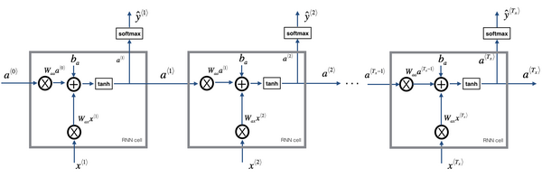
RNN前向传播示意图:
# 使用递归神经网络(RNN)语言模型进行标注图像字幕
# 单个时间步测试前向传播
N, D, H = 3, 10, 4

x = np.linspace(-0.4, 0.7, num=N*D).reshape(N, D)
prev_h = np.linspace(-0.2, 0.5, num=N*H).reshape(N, H)
Wx = np.linspace(-0.1, 0.9, num=D*H).reshape(D, H)
Wh = np.linspace(-0.3, 0.7, num=H*H).reshape(H, H)
b = np.linspace(-0.2, 0.4, num=H)

next_h, _ = rnn_step_forward(x, prev_h, Wx, Wh, b)
expected_next_h = np.asarray([
  [-0.58172089, -0.50182032, -0.41232771, -0.31410098],
  [ 0.66854692,  0.79562378,  0.87755553,  0.92795967],
  [ 0.97934501,  0.99144213,  0.99646691,  0.99854353]])

print('next_h error: ', rel_error(expected_next_h, next_h))
RNN反向传播示意图:
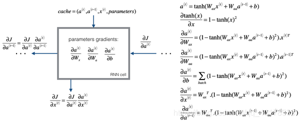
在这个反向传播的过程中,最重要的信息传递或者说最重要的递归运算就是这个从右到左的运算,这也就是为什么这个算法有一个很别致的名字,叫做“通过(穿越)时间反向传播(backpropagation through time)”。取这个名字的原因是对于前向传播,你需要从左到右进行计算,在这个过程中,时刻不断增加。而对于反向传播,你需要从右到左进行计算,就像时间倒流。“通过时间反向传播”,就像穿越时光,这种说法听起来就像是你需要一台时光机来实现这个算法一样。
# 测试单个时间步传播测试反向传播
from cs231n.rnn_layers import rnn_step_forward, rnn_step_backward
np.random.seed(231)
N, D, H = 4, 5, 6
x = np.random.randn(N, D)
h = np.random.randn(N, H)
Wx = np.random.randn(D, H)
Wh = np.random.randn(H, H)
b = np.random.randn(H)

out, cache = rnn_step_forward(x, h, Wx, Wh, b)

dnext_h = np.random.randn(*out.shape)

fx = lambda x: rnn_step_forward(x, h, Wx, Wh, b)[0]
fh = lambda prev_h: rnn_step_forward(x, h, Wx, Wh, b)[0]
fWx = lambda Wx: rnn_step_forward(x, h, Wx, Wh, b)[0]
fWh = lambda Wh: rnn_step_forward(x, h, Wx, Wh, b)[0]
fb = lambda b: rnn_step_forward(x, h, Wx, Wh, b)[0]

dx_num = eval_numerical_gradient_array(fx, x, dnext_h)
dprev_h_num = eval_numerical_gradient_array(fh, h, dnext_h)
dWx_num = eval_numerical_gradient_array(fWx, Wx, dnext_h)
dWh_num = eval_numerical_gradient_array(fWh, Wh, dnext_h)
db_num = eval_numerical_gradient_array(fb, b, dnext_h)

dx, dprev_h, dWx, dWh, db = rnn_step_backward(dnext_h, cache)

print('dx error: ', rel_error(dx_num, dx))
print('dprev_h error: ', rel_error(dprev_h_num, dprev_h))
print('dWx error: ', rel_error(dWx_num, dWx))
print('dWh error: ', rel_error(dWh_num, dWh))
print('db error: ', rel_error(db_num, db))
测试整个数据序列的前向和反向传播
# 测试整个数据序列的前向传播
N, T, D, H = 2, 3, 4, 5

x = np.linspace(-0.1, 0.3, num=N*T*D).reshape(N, T, D)
h0 = np.linspace(-0.3, 0.1, num=N*H).reshape(N, H)
Wx = np.linspace(-0.2, 0.4, num=D*H).reshape(D, H)
Wh = np.linspace(-0.4, 0.1, num=H*H).reshape(H, H)
b = np.linspace(-0.7, 0.1, num=H)

h, _ = rnn_forward(x, h0, Wx, Wh, b)
expected_h = np.asarray([
  [
    [-0.42070749, -0.27279261, -0.11074945,  0.05740409,  0.22236251],
    [-0.39525808, -0.22554661, -0.0409454,   0.14649412,  0.32397316],
    [-0.42305111, -0.24223728, -0.04287027,  0.15997045,  0.35014525],
  ],
  [
    [-0.55857474, -0.39065825, -0.19198182,  0.02378408,  0.23735671],
    [-0.27150199, -0.07088804,  0.13562939,  0.33099728,  0.50158768],
    [-0.51014825, -0.30524429, -0.06755202,  0.17806392,  0.40333043]]])
print('h error: ', rel_error(expected_h, h))

# 测试整个数据序列的反向传播
np.random.seed(231)

N, D, T, H = 2, 3, 10, 5

x = np.random.randn(N, T, D)
h0 = np.random.randn(N, H)
Wx = np.random.randn(D, H)
Wh = np.random.randn(H, H)
b = np.random.randn(H)

out, cache = rnn_forward(x, h0, Wx, Wh, b)

dout = np.random.randn(*out.shape)

dx, dh0, dWx, dWh, db = rnn_backward(dout, cache)

fx = lambda x: rnn_forward(x, h0, Wx, Wh, b)[0]
fh0 = lambda h0: rnn_forward(x, h0, Wx, Wh, b)[0]
fWx = lambda Wx: rnn_forward(x, h0, Wx, Wh, b)[0]
fWh = lambda Wh: rnn_forward(x, h0, Wx, Wh, b)[0]
fb = lambda b: rnn_forward(x, h0, Wx, Wh, b)[0]

dx_num = eval_numerical_gradient_array(fx, x, dout)
dh0_num = eval_numerical_gradient_array(fh0, h0, dout)
dWx_num = eval_numerical_gradient_array(fWx, Wx, dout)
dWh_num = eval_numerical_gradient_array(fWh, Wh, dout)
db_num = eval_numerical_gradient_array(fb, b, dout)

print('dx error: ', rel_error(dx_num, dx))
print('dh0 error: ', rel_error(dh0_num, dh0))
print('dWx error: ', rel_error(dWx_num, dWx))
print('dWh error: ', rel_error(dWh_num, dWh))
print('db error: ', rel_error(db_num, db))
词嵌入
在深度学习系统中,我们通常使用向量表示单词。 词汇表中的每个单词都将与一个向量相关联,并且将与系统的其余部分一起学习这些向量。
# 测试把单词转换为向量
N, T, V, D = 2, 4, 5, 3

x = np.asarray([[0, 3, 1, 2], [2, 1, 0, 3]])
W = np.linspace(0, 1, num=V*D).reshape(V, D)

out, _ = word_embedding_forward(x, W)
expected_out = np.asarray([
 [[ 0.,          0.07142857,  0.14285714],
  [ 0.64285714,  0.71428571,  0.78571429],
  [ 0.21428571,  0.28571429,  0.35714286],
  [ 0.42857143,  0.5,         0.57142857]],
 [[ 0.42857143,  0.5,         0.57142857],
  [ 0.21428571,  0.28571429,  0.35714286],
  [ 0.,          0.07142857,  0.14285714],
  [ 0.64285714,  0.71428571,  0.78571429]]])

print('out error: ', rel_error(expected_out, out))

# 单词嵌入功能的前向传播和反向传播
np.random.seed(231)

N, T, V, D = 50, 3, 5, 6
x = np.random.randint(V, size=(N, T))
W = np.random.randn(V, D)

out, cache = word_embedding_forward(x, W)
dout = np.random.randn(*out.shape)
dW = word_embedding_backward(dout, cache)

f = lambda W: word_embedding_forward(x, W)[0]
dW_num = eval_numerical_gradient_array(f, W, dout)

print('dW error: ', rel_error(dW, dW_num))
在每个时间步上,我们都使用仿射函数将该时间步上的RNN隐藏向量转换为词汇表中每个单词的分数。
np.random.seed(231)

# Gradient check for temporal affine layer
N, T, D, M = 2, 3, 4, 5
x = np.random.randn(N, T, D)
w = np.random.randn(D, M)
b = np.random.randn(M)

out, cache = temporal_affine_forward(x, w, b)

dout = np.random.randn(*out.shape)

fx = lambda x: temporal_affine_forward(x, w, b)[0]
fw = lambda w: temporal_affine_forward(x, w, b)[0]
fb = lambda b: temporal_affine_forward(x, w, b)[0]

dx_num = eval_numerical_gradient_array(fx, x, dout)
dw_num = eval_numerical_gradient_array(fw, w, dout)
db_num = eval_numerical_gradient_array(fb, b, dout)

dx, dw, db = temporal_affine_backward(dout, cache)

print('dx error: ', rel_error(dx_num, dx))
print('dw error: ', rel_error(dw_num, dw))
print('db error: ', rel_error(db_num, db))
在RNN语言模型中,我们在每个时间步都会为词汇表中的每个单词生成一个分数。 我们在每个时间步都知道真实的单词,因此我们使用softmax损失函数来计算每个时间步的损失和梯度。 我们将随着时间的推移对损失进行求和,然后对小批量进行平均。
# 使用softmax损失函数来计算每个时间步的损失和梯度。
# 我们将随着时间的推移对损失进行求和,然后对小批量进行平均。
from cs231n.rnn_layers import temporal_softmax_loss

N, T, V = 100, 1, 10

def check_loss(N, T, V, p):
    x = 0.001 * np.random.randn(N, T, V)
    y = np.random.randint(V, size=(N, T))
    mask = np.random.rand(N, T) <= p
    print(temporal_softmax_loss(x, y, mask)[0])

check_loss(100, 1, 10, 1.0)   # Should be about 2.3
check_loss(100, 10, 10, 1.0)  # Should be about 23
check_loss(5000, 10, 10, 0.1) # Should be about 2.3

# Gradient check for temporal softmax loss
N, T, V = 7, 8, 9

x = np.random.randn(N, T, V)
y = np.random.randint(V, size=(N, T))
mask = (np.random.rand(N, T) > 0.5)

loss, dx = temporal_softmax_loss(x, y, mask, verbose=False)

dx_num = eval_numerical_gradient(lambda x: temporal_softmax_loss(x, y, mask)[0], x, verbose=False)

print('dx error: ', rel_error(dx, dx_num))

# 组合各层以构建图像字幕的模型
N, D, W, H = 10, 20, 30, 40
word_to_idx = {'<NULL>': 0, 'cat': 2, 'dog': 3}
V = len(word_to_idx)
T = 13

model = CaptioningRNN(word_to_idx,
          input_dim=D,
          wordvec_dim=W,
          hidden_dim=H,
          cell_type='rnn',
          dtype=np.float64)

# Set all model parameters to fixed values
for k, v in model.params.items():
    model.params[k] = np.linspace(-1.4, 1.3, num=v.size).reshape(*v.shape)

features = np.linspace(-1.5, 0.3, num=(N * D)).reshape(N, D)
captions = (np.arange(N * T) % V).reshape(N, T)

loss, grads = model.loss(features, captions)
expected_loss = 9.83235591003

print('loss: ', loss)
print('expected loss: ', expected_loss)
print('difference: ', abs(loss - expected_loss))

# 检查梯度
np.random.seed(231)

batch_size = 2
timesteps = 3
input_dim = 4
wordvec_dim = 5
hidden_dim = 6
word_to_idx = {'<NULL>': 0, 'cat': 2, 'dog': 3}
vocab_size = len(word_to_idx)

captions = np.random.randint(vocab_size, size=(batch_size, timesteps))
features = np.random.randn(batch_size, input_dim)

model = CaptioningRNN(word_to_idx,
          input_dim=input_dim,
          wordvec_dim=wordvec_dim,
          hidden_dim=hidden_dim,
          cell_type='rnn',
          dtype=np.float64,
        )

loss, grads = model.loss(features, captions)

for param_name in sorted(grads):
    f = lambda _: model.loss(features, captions)[0]
    param_grad_num = eval_numerical_gradient(f, model.params[param_name], verbose=False, h=1e-6)
    e = rel_error(param_grad_num, grads[param_name])
    print('%s relative error: %e' % (param_name, e))
训练模型
# 训练模型
np.random.seed(231)

small_data = load_coco_data(max_train=50)

small_rnn_model = CaptioningRNN(
          cell_type='rnn',
          word_to_idx=data['word_to_idx'],
          input_dim=data['train_features'].shape[1],
          hidden_dim=512,
          wordvec_dim=256,
        )

small_rnn_solver = CaptioningSolver(small_rnn_model, small_data,
           update_rule='adam',
           num_epochs=50,
           batch_size=25,
           optim_config={
             'learning_rate': 5e-3,
           },
           lr_decay=0.95,
           verbose=True, print_every=10,
         )

small_rnn_solver.train()

# Plot the training losses
plt.plot(small_rnn_solver.loss_history)
plt.xlabel('Iteration')
plt.ylabel('Loss')
plt.title('Training loss history')
plt.show()
# 测试模型
for split in ['train', 'val']:
    minibatch = sample_coco_minibatch(small_data, split=split, batch_size=2)
    gt_captions, features, urls = minibatch
    gt_captions = decode_captions(gt_captions, data['idx_to_word'])

    sample_captions = small_rnn_model.sample(features)
    sample_captions = decode_captions(sample_captions, data['idx_to_word'])

    for gt_caption, sample_caption, url in zip(gt_captions, sample_captions, urls):
        plt.imshow(image_from_url(url))
        plt.title('%s\n%s\nGT:%s' % (split, sample_caption, gt_caption))
        plt.axis('off')
        plt.show()