找tf关于Pruning和quantization的用例较少,正好在做这方面工作,就搬一搬一些官方文档的应用。
下面的代码主要是结合一个官方Mnist的示例和guide文档看看tf的API中是怎么做pruning这一步优化的。
tensorflow/model-optimization--comprehensive_guide
总的思路是: 建baseline model → 加入剪枝操作→ 对比模型大小、acc等变化
其中关注其中如何自定义自己的pruning case和后续quantization等
目录
1.导入一些依赖库,后面似乎没用到tensorboard,暂时注释掉
3.建立一个Baseline模型,并保存权重,方便后续比较性能
4.对整个模型直接magnitude,建立剪枝模型,顺便看看模型前后变化
5.选定某个层进行magnitude(这里选择Dense layer),建立剪枝模型,看看模型变化
import tempfile
import os
import zipfile
import tensorflow as tf
import numpy as np
import tensorflow_model_optimization as tfmot
from tensorflow import keras

#%load_ext tensorboard
1.导入一些依赖库,后面似乎没用到tensorboard,暂时注释掉
#加载MNIST数据集
mnist = keras.datasets.mnist
(train_images, train_labels), (test_images, test_labels) = mnist.load_data()
#将图像像素值规整到[0,1]
train_images = train_images / 255.0
test_images = test_images / 255.0
2.导入Mnist数据集,作简单规整
#建立模型
def setup_model():
    model = keras.Sequential([
        keras.layers.InputLayer(input_shape=(28, 28)),
        keras.layers.Reshape(target_shape=(28, 28, 1)),
        keras.layers.Conv2D(filters=12,kernel_size=(3, 3), activation='relu'),
        keras.layers.MaxPooling2D(pool_size=(2,2)),
        keras.layers.Flatten(),
        keras.layers.Dense(10)
    ])
    return model

#训练分类模型参数
def setup_pretrained_weights():
    model = setup_model()

    model.compile(optimizer = 'adam',
                  loss = tf.keras.losses.SparseCategoricalCrossentropy(from_logits = True),
                  metrics = ['accuracy']
    )

    model.fit(train_images,
              train_labels,
              epochs = 4,
              validation_split = 0.1,
    )

    _, pretrained_weights = tempfile.mkstemp('.tf')

    model.save_weights(pretrained_weights)
    return pretrained_weights
3.建立一个Baseline模型,并保存权重,方便后续比较性能
setup_model()

pretrained_weights = setup_pretrained_weights()

#
Train on 54000 samples, validate on 6000 samples
Epoch 1/4
54000/54000 [==============================] - 7s 133us/sample - loss: 0.2895 - accuracy: 0.9195 - val_loss: 0.1172 - val_accuracy: 0.9685
Epoch 2/4
54000/54000 [==============================] - 5s 99us/sample - loss: 0.1119 - accuracy: 0.9678 - val_loss: 0.0866 - val_accuracy: 0.9758
Epoch 3/4
54000/54000 [==============================] - 5s 100us/sample - loss: 0.0819 - accuracy: 0.9753 - val_loss: 0.0757 - val_accuracy: 0.9787
Epoch 4/4
54000/54000 [==============================] - 6s 103us/sample - loss: 0.0678 - accuracy: 0.9797 - val_loss: 0.0714 - val_accuracy: 0.9815
4.对整个模型直接magnitude,建立剪枝模型,顺便看看模型前后变化
#比较baselin与剪裁模型的差别
base_model = setup_model()
base_model.summary()

base_model.load_weights(pretrained_weights)

model_for_pruning = tfmot.sparsity.keras.prune_low_magnitude(base_model)
model_for_pruning.summary()

#
Model: "sequential_4"
_________________________________________________________________
Layer (type)                 Output Shape              Param #
=================================================================
reshape_4 (Reshape)          (None, 28, 28, 1)         0
_________________________________________________________________
conv2d_4 (Conv2D)            (None, 26, 26, 12)        120
_________________________________________________________________
max_pooling2d_4 (MaxPooling2 (None, 13, 13, 12)        0
_________________________________________________________________
flatten_4 (Flatten)          (None, 2028)              0
_________________________________________________________________
dense_4 (Dense)              (None, 10)                20290
=================================================================
Total params: 20,410
Trainable params: 20,410
Non-trainable params: 0
_________________________________________________________________
Model: "sequential_4"
_________________________________________________________________
Layer (type)                 Output Shape              Param #
=================================================================
prune_low_magnitude_reshape_ (None, 28, 28, 1)         1
_________________________________________________________________
prune_low_magnitude_conv2d_4 (None, 26, 26, 12)        230
_________________________________________________________________
prune_low_magnitude_max_pool (None, 13, 13, 12)        1
_________________________________________________________________
prune_low_magnitude_flatten_ (None, 2028)              1
_________________________________________________________________
prune_low_magnitude_dense_4  (None, 10)                40572
=================================================================
Total params: 40,805
Trainable params: 20,410
Non-trainable params: 20,395
_________________________________________________________________
分析:可以看到各层参数都增多了,其中为了剪枝操作增加的参数是Non-trainable的参数
5.选定某个层进行magnitude(这里选择Dense layer),建立剪枝模型,看看模型变化
为了模块化对某类层进行处理,先def一个函数
#修剪模型的Dense layer
def apply_pruning_to_dense(layer):
    if isinstance(layer, tf.keras.layers.Dense):
        print("Apply pruning to Dense")
        return tfmot.sparsity.keras.prune_low_magnitude(layer)
    return layer
其中tf.keras.models.clone_model是对keras定义的层进行一些改变,具体看一看 官方api
model_for_pruning = tf.keras.models.clone_model(
base_model, clone_function=apply_pruning_to_dense)
model_for_pruning.summary()

#
Apply pruning to Dense
Model: "sequential_4"
_________________________________________________________________
Layer (type)                 Output Shape              Param #
=================================================================
reshape_4 (Reshape)          (None, 28, 28, 1)         0
_________________________________________________________________
conv2d_4 (Conv2D)            (None, 26, 26, 12)        120
_________________________________________________________________
max_pooling2d_4 (MaxPooling2 (None, 13, 13, 12)        0
_________________________________________________________________
flatten_4 (Flatten)          (None, 2028)              0
_________________________________________________________________
prune_low_magnitude_dense_4  (None, 10)                40572
=================================================================
Total params: 40,692
Trainable params: 20,410
Non-trainable params: 20,282
_________________________________________________________________
分析:可以看到只对Dense层加入剪枝操作参数
可能更方便的是根据layer的name在clone_function中去选定剪枝 而不是layer的类型
通过下面的方式可以查看层的name(- - 看summary或者定义layer的时候直接给name比较快吧)
print(base_model.layers[0].name)

#reshape_4
对①Functional的方式和②Sequential中直接用magnitude的方式进行了警告:虽然可读性增加,但精度可能不及上述方式
原因是在定义后再load weights是无效的(- - 应该是无法得到去掉剪枝参数的weight,也就是无法还原模型)
Functional example
# Use `prune_low_magnitude` to make the `Dense` layer train with pruning.
i = tf.keras.Input(shape=(20,))
x = tfmot.sparsity.keras.prune_low_magnitude(tf.keras.layers.Dense(10))(i)
o = tf.keras.layers.Flatten()(x)
model_for_pruning = tf.keras.Model(inputs=i, outputs=o)

model_for_pruning.summary()

Sequential example
# Use `prune_low_magnitude` to make the `Dense` layer train with pruning.
model_for_pruning = tf.keras.Sequential([
  tfmot.sparsity.keras.prune_low_magnitude(tf.keras.layers.Dense(20, input_shape=input_shape)),
  tf.keras.layers.Flatten()
])

model_for_pruning.summary()
6.自定义剪枝操作
通过 tfmot.sparsity.keras.PrunableLayer 自定需要剪枝的参数
常有两种情况:(通常bia的prune会严重降低精度,默认是不会prune的,此处只作示例)
serves two use cases:
- Prune a custom Keras layer
- Modify parts of a built-in Keras layer to prune.
在API的类中有get_prunable_weights()去返回在训练中需要Prune的张量 官方API
class MyDenseLayer(tf.keras.layers.Dense, tfmot.sparsity.keras.PrunableLayer):

  def get_prunable_weights(self):
    # Prune bias also, though that usually harms model accuracy too much.
    return [self.kernel, self.bias]

# Use `prune_low_magnitude` to make the `MyDenseLayer` layer train with pruning.
model_for_pruning = tf.keras.Sequential([
  tfmot.sparsity.keras.prune_low_magnitude(MyDenseLayer(20, input_shape=input_shape)),
  tf.keras.layers.Flatten()
])

model_for_pruning.summary()

#
_________________________________________________________________
Model: "sequential_11"
_________________________________________________________________
Layer (type)                 Output Shape              Param #
=================================================================
prune_low_magnitude_my_dense (None, 28, 10)            583
_________________________________________________________________
flatten_13 (Flatten)         (None, 280)               0
=================================================================
Total params: 583
Trainable params: 290
Non-trainable params: 293
_________________________________________________________________


# Use `prune_low_magnitude` to make the `Dense` layer train with pruning.
i = tf.keras.Input(shape=(28,28))
x = tfmot.sparsity.keras.prune_low_magnitude(tf.keras.layers.Dense(10))(i)
o = tf.keras.layers.Flatten()(x)
model_for_pruning = tf.keras.Model(inputs=i, outputs=o)

model_for_pruning.summary()

#
Model: "model_1"
_________________________________________________________________
Layer (type)                 Output Shape              Param #
=================================================================
input_7 (InputLayer)         [(None, 28, 28)]          0
_________________________________________________________________
prune_low_magnitude_dense_9  (None, 28, 10)            572
_________________________________________________________________
flatten_12 (Flatten)         (None, 280)               0
=================================================================
Total params: 572
Trainable params: 290
Non-trainable params: 282
_________________________________________________________________
分析:可以看到两种方法建模的模型参数,多出来的就是bia的量了
7.Tensorboard 可视化
在训练中添加回调参数 tfmot.sparsity.keras.PruningSummaries 去观测过程中的变量
其中回调参数 tfmot.sparsity.keras.UpdatePruningStep() 是必须的,不然会出错 官方API
base_model = setup_model()
base_model.load_weights(pretrained_weights) # optional but recommended for model accuracy
model_for_pruning = tfmot.sparsity.keras.prune_low_magnitude(base_model)

log_dir = tempfile.mkdtemp()
print(log_dir)#查看保存地址
callbacks = [
    tfmot.sparsity.keras.UpdatePruningStep(),
    # Log sparsity and other metrics in Tensorboard.
    tfmot.sparsity.keras.PruningSummaries(log_dir=log_dir)
]

model_for_pruning.compile(
      loss = tf.keras.losses.SparseCategoricalCrossentropy(from_logits = True),
      optimizer='adam',
      metrics=['accuracy']
)

model_for_pruning.fit(
    train_images,
    train_labels,
    callbacks=callbacks,
    epochs=2,
)
给一下这个model的summary方便看name和参数结构
_________________________________________________________________
Layer (type)                 Output Shape              Param #
=================================================================
prune_low_magnitude_reshape_ (None, 28, 28, 1)         1
_________________________________________________________________
prune_low_magnitude_conv2d_2 (None, 26, 26, 12)        230
_________________________________________________________________
prune_low_magnitude_max_pool (None, 13, 13, 12)        1
_________________________________________________________________
prune_low_magnitude_flatten_ (None, 2028)              1
_________________________________________________________________
prune_low_magnitude_dense_2  (None, 10)                40572
=================================================================
Total params: 40,805
Trainable params: 20,410
Non-trainable params: 20,395
_________________________________________________________________
终于到可视化这一步了!
tensorboard --logdir=log_dirScalars中有epoch_accuracy、epoch_loss(很简单的两个point,图略) 重点:acc比修剪前的高(0.97 ↑ 0.98)
还有两个层的稀疏度与阈值变化图,重点看看这两个
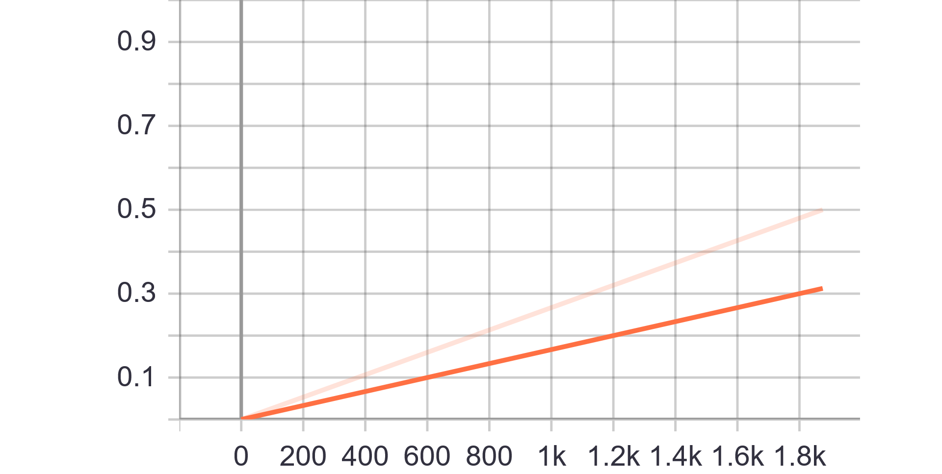
分析:只是简单地用了 model_for_pruning = tfmot.sparsity.keras.prune_low_magnitude(base_model)
所以可以看到随着训练step by step最终到达0.5稀疏度的mask(=0)
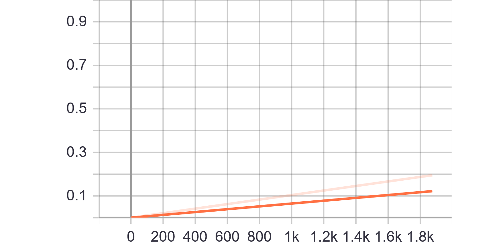
分析:阈值逐步增大去筛选权重小的参数,最后一个point的value是0.1952
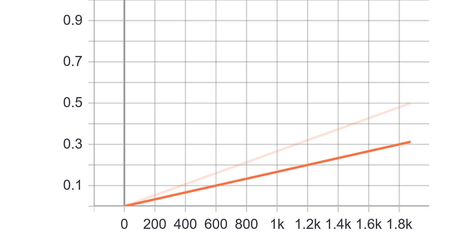
分析:跟conv2d的一致
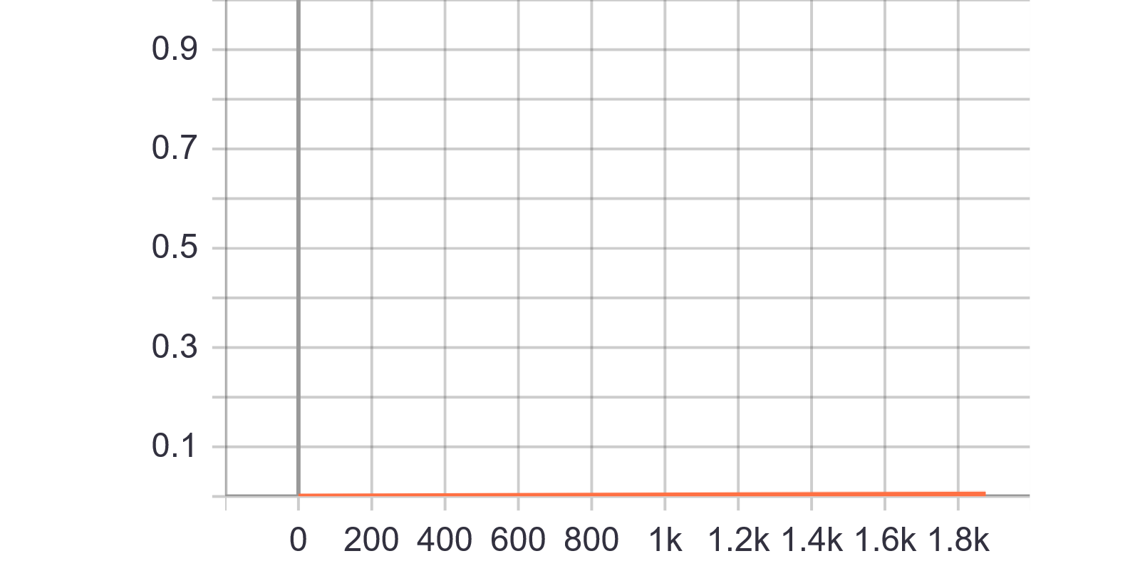
分析:阈值几乎为0就把稀疏度冲上了0.5,证实了Dense Layer有大量冗余信息存在的先验知识,即Dense层可以大幅度扔掉!
8.保存模型 比较精度、模型大小
常见错误:strip_pruning和应用标准压缩算法(例如通过gzip)都是必需的,以查看修剪的压缩优势。
说人话:strip_pruning或者用gzip之类的压缩掉有0的参数得到的模型大小来观测稀疏效果
先整一个计算模型大小模块:
#获得模型权重大小
def get_gzipped_model_size(model):
    _, keras_file = tempfile.mkstemp('.h5')
    model.save(keras_file, include_optimizer=False)

    _, zipped_file = tempfile.mkstemp('.zip')
    with zipfile.ZipFile(zipped_file, 'w', compression=zipfile.ZIP_DEFLATED) as f:
        f.write(keras_file)
    return os.path.getsize(zipped_file)
model_for_export = tfmot.sparsity.keras.strip_pruning(model_for_pruning)
print("final model")
model_for_export.summary()
print("\n")
print("Size of gzipped pruned model without stripping: %.2f bytes" % (get_gzipped_model_size(model_for_pruning)))
print("Size of gzipped pruned model with stripping: %.2f bytes" % (get_gzipped_model_size(model_for_export)))
#
_________________________________________________________________
Layer (type) Output Shape Param #
=================================================================
reshape_3 (Reshape) (None, 28, 28, 1) 0
_________________________________________________________________
conv2d_3 (Conv2D) (None, 26, 26, 12) 120
_________________________________________________________________
max_pooling2d_3 (MaxPooling2 (None, 13, 13, 12) 0
_________________________________________________________________
flatten_3 (Flatten) (None, 2028) 0
_________________________________________________________________
dense_3 (Dense) (None, 10) 20290
=================================================================
Total params: 20,410
Trainable params: 20,410
Non-trainable params: 0
_________________________________________________________________
Size of gzipped pruned model without stripping: 55570.00 bytes
Size of gzipped pruned model with stripping: 48518.00 bytes我们可以看到稀疏操作的参数都通过strip_pruning去掉,恢复到了baseline的样子
模型大概有个×1.15的压缩,精度上面测过略有提升,不再赘述。
中间有个callback的应用跳过了,大致和keras中的callback用法差不多,一些on_epoch和on_train之类的函数可以用作调试点
提高修剪模型的准确性Tips:
- 修剪模型时学习率不宜过高或过低(- - 有点废话的意思) 把修剪视为一个超参数;
- 作为快速测试,尝试设置begin_step=0去剪枝以达成稀疏度目标,这样可能得到好的结果;
- 把握剪枝频率(参数frequency),让模型有时间recover;
- 在Define model下去做自己的case。
Common mistake:
- 为了保留剪枝操作,须用.h5去load model而不是load weights;
- 剪枝结束去掉剪枝参数,用Strip_pruning或者gzip的压缩方法的一个就好了。