一、支持向量机
支持向量机的基本思想是SVM从线性可分情况下的最优分类面发展而来。最优分类面就是要求分类线不但能将两类正确分开(训练错误率为0),且使分类间隔最大。SVM考虑寻找一个满足分类要求的超平面,并且使训练集中的点距离分类面尽可能的远,也就是寻找一个分类面使它两侧的空白区域(margin)最大。(SVM算法就是为找到距分类样本点间隔最大的分类超平面
(ω,b)过两类样本中离分类面最近的点,且平行于最优分类面的超平面上H1,H2的训练样本就叫支持向量。)

上图中直线
(ω∗.x)+b∗=0是空间R2上的分划线。直线(ω∗.x)+b∗=1和(ω∗.x)+b∗=−1是两条支持直线.属于正类的非支持向量一定位于对应1的支持直线的一侧(包含边界线),属于负类的非支持向量一定位于对应-1的支持直线的一侧(包含边界线).而属于正类的支持向量和属于负类的支持向量分别位于上述两条支持直线上由此可以体会“支持向量”一词的由来。(如图中的红框框里面的点即是支持向量)
1.线性支持向量机
给定线性可分(不可分)的训练数据集,通过硬(软)间隔最大化或者等价的
的求解相应的凸二次规划问题学习得到的分离超平面为:
ω∗x+b=0
以及相应的分类决策函数:
f(x)=sign(ω∗x)+bf(x)=sign(ω∗x)+b
2.非线性支持向量机
从非线性分类训练集,通过核函数与软间隔最大化,或者凸二次优化,学习得到的分类决策函数
f(x)=sign(i=1∑NαiyiK(x,xi)+b)
其中,K(x,z)是正定核函数。
二、支持向量机重要概念
1.函数间隔
定义超平面(ω,b)关于样本点(xi,yi)的函数间隔是γi^=yi(w∗xi+b);超平面ω,b关于训练集T的函数间隔为:超平面(ω,b)与所有样本点(xi,yi)的函数间隔最小值:
γ^=i=1,2...Nminγi^
2.几何间隔
定义超平面(ω,b)关于样本点(xi,yi)的几何间隔是γi=yi(∥ω∥ω∗xi+∥ω∥b);
超平面(ω,b)关于训练数据集T的几何间隔是:超平面(ω,b)与所有样本点(xi,yi)的几何间隔最小值:
γ=i=1,2...Nminγi^
- 几何间隔是为样本点到超平面的带符号距离,当样本被正确分类时,即为样本点到超平面的距离
3.核函数
从输入空间χ(欧式空间Rn的子集或者离散集合)到特征空间H(希尔伯特空间)的映射:ϕ(x):χ⇒H;使得对所有的x,z∈χ,函数K(x,z)满足条件K(x,z)=ϕ(x)∗ϕ(z),则称K(x,z)为核函数,ϕ(x)为映射函数。
三、拉格朗日对偶性
1.原始问题
假设f(x),ci(x),hj(x)是定义在Rn上的连续可微函数,考虑约束最优化问题:
⎩⎪⎨⎪⎧x∈Rnminf(x) ①s.t.ci(x)≤0,i=1,2,3,......k ②hj(x)=0,j=1,2,3,......l ③
则该约束最优化问题为原始问题或者原始最优化问题。
在求解该最优化问题时,首先引入广义拉格朗日函数(generalized Lagrange function)
L(x,α,β)=f(x)+i=1∑kαici(x)+j=1∑lβjhj(x)拉格朗日乘子,且αi≥0。考虑x的函数θp(x)=α,β,αi≥0maxL(x,α,β)=α,β,αi≥0max[f(x)+i=1∑kαici(x)+j=1∑lβjhj(x)]
如果x违反约束条件,即存在xi使得ci(xi)>0或者存在xj使得hj(xj)=0,则有θp(x)=α,β,αi≥0maxL(x,α,β)=+∞
1.若xi使约束条件ci(x)>0,则令αi→+∞,使得αici(x)→+∞;2.若xj使得约束条件hj(xj)=0,则令βj→+∞,使得βjhj(xj)→∞βjhj(xj)→∞,同时令其余α,β均取0,可得θp(x)=+∞。
所以有:
θp(x)={f(x) x满足约束条件+∞ 其他
原始最优化问题转换为:
P∗=xminα,β,αi≥0maxL(x,α,β);P∗定义为原始问题的最优值。
2.对偶问题
定义:θD=xminL(x,α,β)。
再考虑对θD=xminL(x,α,β)的极大化,即α,β,αi≥0maxθD=α,β,αi≥0maxxminL(x,α,β)。
问题α,β,αi≥0maxxminL(x,α,β)成为广义拉格朗日函数的极大极小问题。
将广义拉格朗日函数的极大极小问题表示为约束最优化问题:
α,β,αi≥0maxθD=α,β,αi≥0maxxminL(x,α,β)
s.t.αi≥0
称为原始问题的对偶问题,定义对偶问题的最优值为:d∗=α,β,αi≥0maxθD
3.原始问题与对偶问题的关系
定理1: 若原始问题与对偶问题都有最优值,则
d∗=α,β,αi≥0maxxminL(x,α,β)≤xminα,β,αi≥0maxL(x,α,β)=P∗。
定理2:考虑原始问题与对偶问题,假设函数f(x)和ci(x)是凸函数,hj(x)是仿射函数;并且假设不等式约束ci(x)是严格可行的,即存在x,对所有i有ci(x)<0,则存在x∗,α∗,β∗,使得x∗是原始问题的解,α∗,β∗是对偶问题的解,并且P∗=L(x,α,β)。
- 在满足约束条件下,该定理保证了对偶问题求的最优解,既是对原始问题求的最优值。
定理3:考虑原始问题与对偶问题,假设函数f(x)和ci(x)是凸函数,hj(x)是仿射函数;并且假设不等式约束ci(x)是严格可行的,则x∗和α∗,β∗分别原始问题和对偶问题解的充分必要条件是x∗,α∗,β∗满足KKT条件:
▽xL(x∗,α∗,β∗)=0▽αLx∗,α∗,β∗)=0▽βLx∗,α∗,β∗)=0
αi∗ci(x∗)=0,i=1,2,……,k这条重要,在优化α,
选择第一个变量的依据是违反KKT条件,就是违反了这一条ci(x∗)≤0,i=1,2,……,kαi∗≥0,i=1,2,……,khj(xj∗)=0,j=1,2,……,l
4.目标函数
SVM 算法的分类思想是求得一个几何间隔最大的分离超平面,即最大间隔分离超平面,可表示为以下约束问题:
ω,bmaxγs.t. yi(∥ω∥ω∗xi+∥ω∥b)≥γ,i=1,2,…N
最大化分离超平面与训练数据集的几何间隔γ,约束条件保证了所有样本点与分离超平面的几何间隔至少为γ。根据几何间隔与函数间隔的关系,γ=∥ω∥γ^,上述问题可转换为:
ω,bmax∥ω∥γ^s.t.yi(ω∗xi+b)≥γ^,i=1,2,…N
由于函数间隔γ^的取值不影响最优化问题,可取γ^=1(线性可分支持向量机)。对∥ω∥1求极大值,可转换为求∥ω∥2的极小值。但在线性不可分训练集中,某些样本点可能不满足函数间隔大于等于1的约束条件。所以,对每个样本点引入一个松弛变量ξ≥0。(在机器学习实战中,ξ称为容错率)因此上述约束条件改为:s.t.yi(ω∗xi+b)≥1−ξi,i=1,2,…N
于是,可得目标函数,即最优化问题转换为:ω,b,ξmin21∥ω∥2+Ci=1∑Nξi ; s.t.yi(ω∗xi+b)≥1−ξi这一项就是拉格朗日对偶性中的ci(x)ξi≥0,i=1,2,……,NC≥0是惩罚参数,C值大时对误分类的惩罚增加,C值小时对误分类的惩罚减小(boosting的原理也是惩罚误分类点(这是SVM和boosting的相似处))。最小化目标函数,一方面使间隔尽量大(21∥ω∥2尽量小),同时,使误分类点的个数尽量减小。C是调节二者的系数。当ξi=0时,为线性可分SVM的参数优化模型。

约束条件①②③④⑤
⎩⎪⎪⎪⎪⎪⎪⎨⎪⎪⎪⎪⎪⎪⎧αi(yi(ω∗x+b)−1+ξi)=0 ①C−αi−μi=0 ②αi≥0 ③μi≥0 ④αiμi=0 ⑤
αi(yi(ω∗x+b)−1+ξi)=0及αi的取值不同,软间隔的支持向量xi有4种可能:若αi<C,则ξi=0,该样本点恰好落在间隔边界上,如点A若αi=C,0<ξi<1,则分类正确,该样本落在间隔边界和分离超平面之间,如点B若αi=C,ξi=1,则该样本落在分离超平面之间,如点M若αi=C,ξi>1,则该样本落在分离超平面误分的一侧;如点N
四、sklearn中的SVM
1.准备一个简单二分类数据集
import numpy as np
import matplotlib.pyplot as plt
from sklearn import datasets
iris = datasets.load_iris()
x = iris.data
y = iris.target
# 只做一个简单的二分类
x = x[y<2, :2]
y = y[y<2]
plt.scatter(x[y==0, 0], x[y==0, 1])
plt.scatter(x[y==1, 0], x[y==1, 1])
plt.show()

2.实现svm,先使用一个比较大的C
# 标准化数据
from sklearn.preprocessing import StandardScaler
from sklearn.svm import LinearSVC
standardscaler = StandardScaler()
standardscaler.fit(x)
x_standard = standardscaler.transform(x)
svc = LinearSVC(C=1e9)
svc.fit(x_standard, y)
def plot_decision_boundary(model, axis):
    x0, x1 = np.meshgrid(np.linspace(axis[0], axis[1], int((axis[1] - axis[0])*100)).reshape(1, -1),np.linspace(axis[2], axis[3], int((axis[3] - axis[2])*100)).reshape(1, -1),)
    x_new = np.c_[x0.ravel(), x1.ravel()]
    y_predict = model.predict(x_new)
    zz = y_predict.reshape(x0.shape)
    from matplotlib.colors import ListedColormap
    custom_cmap = ListedColormap(['#EF9A9A','#FFF59D','#90CAF9'])
plt.contourf(x0, x1, zz, linewidth=5, cmap=custom_cmap)
plot_decision_boundary(svc, axis=[-3, 3, -3, 3])
plt.scatter(x_standard[y==0, 0], x_standard[y==0, 1], color='red')
plt.scatter(x_standard[y==1, 0], x_standard[y==1, 1], color='blue')
plt.show()

3.使用一个比较小的C,对比C取不同值的效果
svc2 = LinearSVC(C=0.01)
svc2.fit(x_standard, y)
plot_decision_boundary(svc2, axis=[-3, 3, -3, 3])
plt.scatter(x_standard[y==0, 0], x_standard[y==0, 1], color='red')
plt.scatter(x_standard[y==1, 0], x_standard[y==1, 1], color='blue')
plt.show()

对比两幅图可以发现,当C较小时,误将一个红色的点分到蓝色当中,这也再次验证了当C越小,就意味着有更大的容错空间
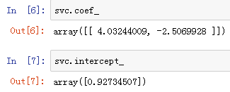
4.查看线性SVM的截距和系数
svc.coef_
svc.intercept_
5.画出除了决策边界以外的两条跟支持向量相关的直线
def plot_svc_decision_boundary(model, axis):
    x0, x1 = np.meshgrid(np.linspace(axis[0], axis[1], int((axis[1] - axis[0])*100)).reshape(1, -1),np.linspace(axis[2], axis[3], int((axis[3] - axis[2])*100)).reshape(1, -1),)
    x_new = np.c_[x0.ravel(), x1.ravel()]
    y_predict = model.predict(x_new)
    zz = y_predict.reshape(x0.shape)
    from matplotlib.colors import ListedColormap
    custom_cmap = ListedColormap(['#EF9A9A', '#FFF59D', '#90CAF9'])
    plt.contourf(x0, x1, zz, linewidth=5, cmap=custom_cmap)
    w = model.coef_[0]
    b = model.intercept_[0]
    # w0*x0 + w1*x1 + b = 0
    # x1 = -w0/w1 * x0 - b/w1
    plot_x = np.linspace(axis[0], axis[1], 200)
    up_y = -w[0]/w[1] * plot_x - b/w[1] + 1/w[1]
    down_y = -w[0]/w[1] * plot_x - b/w[1] - 1/w[1]
    up_index = (up_y >= axis[2]) & (up_y <= axis[3])
    down_index = (down_y >= axis[2]) & (down_y <= axis[3])
    plt.plot(plot_x[up_index], up_y[up_index], color='black')
    plt.plot(plot_x[down_index], down_y[down_index], color='black')
plot_svc_decision_boundary(svc, axis=[-3, 3, -3, 3])
plt.scatter(x_standard[y==0, 0], x_standard[y==0, 1], color='red')
plt.scatter(x_standard[y==1, 0], x_standard[y==1, 1], color='blue')
plt.show()

plot_svc_decision_boundary(svc2, axis=[-3, 3, -3, 3])
plt.scatter(x_standard[y==0, 0], x_standard[y==0, 1], color='red')
plt.scatter(x_standard[y==1, 0], x_standard[y==1, 1], color='blue')
plt.show()

svc3 = LinearSVC(C=0.1)
svc3.fit(x_standard, y)
# 从上述结果可以看出sklearn中对于svm封装的linearSVC默认对于多分类使用ovr,L2正则。
plot_svc_decision_boundary(svc3, axis=[-3, 3, -3, 3])
plt.scatter(x_standard[y==0, 0], x_standard[y==0, 1], color='red')
plt.scatter(x_standard[y==1, 0], x_standard[y==1, 1], color='blue')
plt.show()

五、SVM中使用多项式特征
1.svm解决非线性问题,先生成数据集
import numpy as np
import matplotlib.pyplot as plt
from sklearn import datasets
x, y = datasets.make_moons()
#x.shape
#y.shape
plt.scatter(x[y==0, 0], x[y==0, 1])
plt.scatter(x[y==1, 0], x[y==1, 1])
plt.show()

2.给数据添加一些随机噪声
x, y = datasets.make_moons(noise=0.15, random_state=666)
plt.scatter(x[y==0, 0], x[y==0, 1])
plt.scatter(x[y==1, 0], x[y==1, 1])
plt.show()

from sklearn.preprocessing import PolynomialFeatures, StandardScaler
from sklearn.svm import LinearSVC
from sklearn.pipeline import Pipeline
def PolynomiaSVC(degree, C=1.0):
    return Pipeline([('poly', PolynomialFeatures(degree=degree)),('std_scale', StandardScaler()),('linear_svc', LinearSVC(C=C))])
poly_svc = PolynomiaSVC(degree=3)
poly_svc.fit(x, y)
def plot_decision_boundary(model, axis):
    x0, x1 = np.meshgrid(np.linspace(axis[0], axis[1], int((axis[1] - axis[0])*100)).reshape(1, -1),np.linspace(axis[2], axis[3], int((axis[3] - axis[2])*100)).reshape(1, -1),)
    x_new = np.c_[x0.ravel(), x1.ravel()]
    y_predict = model.predict(x_new)
    zz = y_predict.reshape(x0.shape)
    from matplotlib.colors import ListedColormap
    custom_cmap = ListedColormap(['#EF9A9A', '#FFF59D', '#90CAF9'])
    plt.contourf(x0, x1, zz, linewidth=5, cmap=custom_cmap)
plot_decision_boundary(poly_svc, axis=[-1.5, 2.5, -1.0, 1.5])
plt.scatter(x[y==0, 0], x[y==0, 1])
plt.scatter(x[y==1, 0], x[y==1, 1])
plt.show()

除了使用这种增加多项式特征之后再给入线性svc中之外,还有一种方法可以实现类似的功能
from sklearn.svm import SVC
# 这种方法训练的过程并不完全是先将数据进行标准化,再使用linearSVC这么一个过程
# SVC中默认的C=0
def PolynomiaKernelSVC(degree, C=1.0):
    return Pipeline([('std_scale', StandardScaler()),('kernel_svc', SVC(kernel='poly', degree=degree, C=C))])# poly代表多项式特征
poly_kernel_svc = PolynomiaKernelSVC(degree=3)
poly_kernel_svc.fit(x, y)
plot_decision_boundary(poly_svc, axis=[-1.5, 2.5, -1.0, 1.5])
plt.scatter(x[y==0, 0], x[y==0, 1])
plt.scatter(x[y==1, 0], x[y==1, 1])
plt.show()

是svm中kernel函数
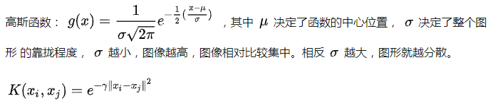
六、高斯核函数
高斯核函数的目的就是将每一个样本点映射到一个无穷维的特征空间。实质上就是把一个
m∗n维的数据映射成了
m∗m的数据。由于理论上数据量可以是无穷维,所以说是映射到一个无穷维空间中。

1.通过高斯核函数映射来更加直观地理解整个映射的过程
import numpy as np
import matplotlib.pyplot as plt
x = np.arange(-4, 5, 1)
y = np.array((x >= -2) & (x <= 2), dtype='int')
# array([0, 0, 1, 1, 1, 1, 1, 0, 0])
plt.scatter(x[y==0], [0] * len(x[y==0]))
plt.scatter(x[y==1], [0] * len(x[y==1]))
plt.show()

def gaussian(x, l):
    gamma = 1.0
    return np.exp(-gamma *(x-l)**2)
l1, l2 = -1, 1
x_new = np.empty((len(x), 2))
for i,data in enumerate(x):
    x_new[i, 0] = gaussian(data, l1)
    x_new[i, 1] = gaussian(data, l2)
plt.scatter(x_new[y==0, 0], x_new[y==0, 1])
plt.scatter(x_new[y==1, 0], x_new[y==1, 1])
plt.show()

真正的高斯核函数实现的过程中并不是固定的landmark,而是对于每一个数据点都是landmark

gamma越大,高斯分布越宽;gamma越小,高斯分布越窄。
2.使用sklearn中封装的高斯核函数
最大化分离超平面与训练数据集的几何间隔gamma(γ)=1.0时
import numpy as np
import matplotlib.pyplot as plt
from sklearn import datasets
x, y = datasets.make_moons(noise=0.15, random_state=666)
from sklearn.preprocessing import StandardScaler
from sklearn.svm import SVC
from sklearn.pipeline import Pipeline
def RBFKernelSVC(gamma=1.0):
    return Pipeline([('std_scale', StandardScaler()),('svc', SVC(kernel='rbf', gamma=gamma))])
svc = RBFKernelSVC(gamma=1.0)
svc.fit(x, y)
def plot_decision_boundary(model, axis):
    x0, x1 = np.meshgrid(np.linspace(axis[0], axis[1], int((axis[1] - axis[0])*100)).reshape(1, -1),np.linspace(axis[2], axis[3], int((axis[3] - axis[2])*100)).reshape(1, -1),)
    x_new = np.c_[x0.ravel(), x1.ravel()]
    y_predict = model.predict(x_new)
    zz = y_predict.reshape(x0.shape)
    from matplotlib.colors import ListedColormap
    custom_cmap = ListedColormap(['#EF9A9A', '#FFF59D', '#90CAF9'])
    plt.contourf(x0, x1, zz, linewidth=5, cmap=custom_cmap)
plot_decision_boundary(svc, axis=[-1.5, 2.5, -1.0, 1.5])
plt.scatter(x[y==0, 0], x[y==0, 1])
plt.scatter(x[y==1, 0], x[y==1, 1])
plt.show()

- 最大化分离超平面与训练数据集的几何间隔gamma(γ)=100时
svc_gamma100 = RBFKernelSVC(gamma=100)
svc_gamma100.fit(x, y)
plot_decision_boundary(svc_gamma100, axis=[-1.5, 2.5, -1.0, 1.5])
plt.scatter(x[y==0, 0], x[y==0, 1])
plt.scatter(x[y==1, 0], x[y==1, 1])
plt.show()

- 最大化分离超平面与训练数据集的几何间隔gamma(γ)=10时
svc_gamma10 = RBFKernelSVC(gamma=10)
svc_gamma10.fit(x, y)
plot_decision_boundary(svc_gamma10, axis=[-1.5, 2.5, -1.0, 1.5])
plt.scatter(x[y==0, 0], x[y==0, 1])
plt.scatter(x[y==1, 0], x[y==1, 1])
plt.show()

- 最大化分离超平面与训练数据集的几何间隔gamma(γ)=0.1时
svc_gamma01 = RBFKernelSVC(gamma=0.1)
svc_gamma01.fit(x, y)
plot_decision_boundary(svc_gamma01, axis=[-1.5, 2.5, -1.0, 1.5])
plt.scatter(x[y==0, 0], x[y==0, 1])
plt.scatter(x[y==1, 0], x[y==1, 1])
plt.show()

gamma相当于是在调节模型的复杂度,gammma越小模型复杂度越低,gamma越高模型复杂度越高。因此需要调节超参数gamma平衡过拟合和欠拟合。
七、SVM解决回归问题
1.在sklearn中实现SVM解决回归问题(在margin区域内的点越多越好)
import numpy as np
import matplotlib.pyplot as plt
from sklearn import datasets
boston = datasets.load_boston()
x = boston.data
y = boston.target
from sklearn.model_selection import train_test_split
x_train, x_test, y_train, y_test = train_test_split(x, y, random_state=888)
from sklearn.svm import SVR
from sklearn.svm import LinearSVR
from sklearn.preprocessing import StandardScaler
from sklearn.pipeline import Pipeline
def StandardLinearSVR(epsilon=0.1):
    return Pipeline([
        ('std_scale', StandardScaler()),
        # C, kernel, 等超参数需要调节
        ('linear_svr', LinearSVR(epsilon=epsilon))])
svr = StandardLinearSVR()
svr.fit(x_train, y_train)
svr.score(x_test, y_test)
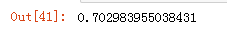
由上图输出结果可知,准确率0.703其实并不高,这是因为使用了默认的参数,超参数epsilon,C,kernel等的设置,包括使用交叉验证等等,可以逐步提高准确率。
参考文献