一、获取历史行情数据
使用tushare库进行数据获取
http://tushare.org/trading.html#id2
import tushare as ts

ts.get_hist_data('600848') #一次性获取全部日k线数据
open high close low volume p_change ma5 \
date
2012-01-11 6.880 7.380 7.060 6.880 14129.96 2.62 7.060
2012-01-12 7.050 7.100 6.980 6.900 7895.19 -1.13 7.020
2012-01-13 6.950 7.000 6.700 6.690 6611.87 -4.01 6.913
2012-01-16 6.680 6.750 6.510 6.480 2941.63 -2.84 6.813
2012-01-17 6.660 6.880 6.860 6.460 8642.57 5.38 6.822
2012-01-18 7.000 7.300 6.890 6.880 13075.40 0.44 6.788
2012-01-19 6.690 6.950 6.890 6.680 6117.32 0.00 6.770
2012-01-20 6.870 7.080 7.010 6.870 6813.09 1.74 6.832
ma10 ma20 v_ma5 v_ma10 v_ma20 turnover
date
2012-01-11 7.060 7.060 14129.96 14129.96 14129.96 0.48
2012-01-12 7.020 7.020 11012.58 11012.58 11012.58 0.27
2012-01-13 6.913 6.913 9545.67 9545.67 9545.67 0.23
2012-01-16 6.813 6.813 7894.66 7894.66 7894.66 0.10
2012-01-17 6.822 6.822 8044.24 8044.24 8044.24 0.30
2012-01-18 6.833 6.833 7833.33 8882.77 8882.77 0.45
2012-01-19 6.841 6.841 7477.76 8487.71 8487.71 0.21
2012-01-20 6.863 6.863 7518.00 8278.38 8278.38 0.23二、标准化
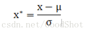
使用零均值归一化
这种方法给予原始数据的均值(mean)和标准差(standard deviation)进行数据的标准化。经过处理的数据符合标准正态分布,即均值为0,标准差为1。
三、相似度计算
相似性使用余弦距离

我们可以通过夹角的大小,来判断向量的相似程度。夹角越小,就代表越相似。将某天行情开盘价,收盘价等指标想象成N维空间上的一个向量,则它和某个样本夹角越小,则它们越相似。
四、绘制图像
使用2020年7月15日收盘行情,计算历史上与哪些天行情最相似,并绘制结果如下:

从图中看到除去2020年7月15日附近行情,跟2019年3月上旬和4月上旬行情很相似。
五、分析


python代码
# @Time : 2020/7/16
# @Author : 大太阳小白
# @Software: PyCharm
# @blog:https://blog.csdn.net/weixin_41579863
import tushare as ts
import pandas as pd
import matplotlib.pyplot as plt
import numpy as np
top = 10
# 获取上证指数,并保存
# data = ts.get_hist_data('sh')
# print(data)
# data.to_excel('data.xlsx')
data = pd.read_excel('data.xlsx')
# 取出当天行情,要跟历史进行对比
today_quote = data.values[0, 1:]
his_data = data.values[1:, 1:].astype(np.float32)
# 使用零均值归一化,所以要计算历史数据的标准差和均值
quote_std = np.std(his_data, axis=0)
quote_mean = np.std(his_data, axis=0)
# 进行数据归一化
normal_his_data = (his_data - quote_mean)/quote_std
normal_today_quote = (today_quote - quote_mean)/quote_std
sim_array = np.zeros((len(normal_his_data), 1))
for index, normal_his_data_item in enumerate(normal_his_data):
    # 遍历计算余弦距离
    a_b = np.mat(normal_today_quote)*np.mat(normal_his_data_item).T
    a = np.mat(normal_today_quote) * np.mat(normal_today_quote).T
    b = np.mat(normal_his_data_item) * np.mat(normal_his_data_item).T
    sim = a_b.A.astype(np.float32)/(np.sqrt(a.A.astype(np.float32)) * np.sqrt(b.A.astype(np.float32)))
    sim_array[index] = sim[0][0]
# 对结果进行降序排序,并获取topN的索引
top_n = np.argsort(sim_array, axis=0)[::-1][:top]
# 绘图
fig = plt.figure()
for top_index, value in enumerate(top_n):
    ax1 = fig.add_subplot(top/2, 2, top_index+1)
    ax1.set_title(data.values[value+1,0][0])
    row = value[0]
    y = his_data[row:row+20, 2][::-1]
    x = range(len(y))
    ax1.plot(x,  y)
plt.show()