本文参考链接:https://www.yiibai.com/pandas
三种 pandas 数据结构的创建和数据获取
系列 pandas.Series
创建空系列
>>> import pandas as pd
>>> s = pd.Series()
>>> s
Series([], dtype: float64)

从ndarray创建一个系列
>>> import numpy as np
>>> data = np.array(['a', 'b', 'c', 'd'])
>>> pd.Series(data)
0    a
1    b
2    c
3    d
dtype: object
>>> pd.Series(data, index=[100, 101, 102, 103])
100    a
101    b
102    c
103    d
dtype: object

从字典创建一个系列
>>> data = {'a':0, 'b':1, 'c':2}
>>> data
{'a': 0, 'b': 1, 'c': 2}
>>> pd.Series()
Series([], dtype: float64)
>>> pd.Series(data)
a    0
b    1
c    2
dtype: int64
>>> pd.Series(data, index=['b','c','d','a'])
b    1.0
c    2.0
d    NaN
a    0.0
dtype: float64


从标量创建一个系列
>>> pd.Series(5)
0    5
dtype: int64
>>> pd.Series(5, index=[0, 1, 2, 3])
0    5
1    5
2    5
3    5
dtype: int64

通过索引访问系列数据(类似于列表操作)
>>> s = pd.Series([1,2,3,4,5],index = ['a','b','c','d','e'])
>>> s
a    1
b    2
c    3
d    4
e    5
dtype: int64
>>> s[0]
1
>>> s[:3]
a    1
b    2
c    3
dtype: int64
>>> s[-3:]
c    3
d    4
e    5
dtype: int64

通过索引标签访问系列数据
>>> s['a']
1
>>> s[['a', 'b', 'c']]
a    1
b    2
c    3
dtype: int64

-------------------------------------------------------------------------------------------
数据帧 pandas.DataFrame
创建空数据帧
>>> pd.DataFrame()
Empty DataFrame
Columns: []
Index: []
>>> data = [1,2,3,4,5]
>>> pd.DataFrame(data)
   0
0  1
1  2
2  3
3  4
4  5
>>> data = [['Alex',10],['Bob',12],['Clarke',13]]
>>> pd.DataFrame(data)
        0   1
0    Alex  10
1     Bob  12
2  Clarke  13
>>> pd.DataFrame(data, index=['a', 'b', 'c'], columns=['Name', 'Age'])
     Name  Age
a    Alex   10
b     Bob   12
c  Clarke   13
>>> pd.DataFrame(data, index=['a', 'b', 'c'], columns=['Name', 'Age'], dtype=float)
     Name   Age
a    Alex  10.0
b     Bob  12.0
c  Clarke  13.0

从字典来创建DataFrame
>>> data = {'Name':['Tom', 'Jack', 'Steve', 'Ricky'],'Age':[28,34,29,42]}
>>> data
{'Name': ['Tom', 'Jack', 'Steve', 'Ricky'], 'Age': [28, 34, 29, 42]}
>>> pd.DataFrame(data)
   Age   Name
0   28    Tom
1   34   Jack
2   29  Steve
3   42  Ricky
>>> pd.DataFrame(data, index=[1, 2, 3, 4])
   Age   Name
1   28    Tom
2   34   Jack
3   29  Steve
4   42  Ricky

从字典列表来创建DataFrame
>>> data = [{'a': 1, 'b': 2},{'a': 5, 'b': 10, 'c': 20}]
>>> data
[{'a': 1, 'b': 2}, {'a': 5, 'b': 10, 'c': 20}]
>>> pd.DataFrame(data)
   a   b     c
0  1   2   NaN
1  5  10  20.0
# 可以在创建时自己指定行索引和列索引
>>> pd.DataFrame(data, index=['first', 'second'])
        a   b     c
first   1   2   NaN
second  5  10  20.0

从系列的字典来创建DataFrame
>>> d = {'one' : pd.Series([1, 2, 3], index=['a', 'b', 'c']),
      'two' : pd.Series([1, 2, 3, 4], index=['a', 'b', 'c', 'd'])}
>>> pd.DataFrame(d)
   one  two
a  1.0    1
b  2.0    2
c  3.0    3
d  NaN    4
>>> df = pd.DataFrame(d)
# 数据帧应该是列优先的,所以df['one']能正常执行获取到数据
>>> df['one']
a    1.0
b    2.0
c    3.0
d    NaN
Name: one, dtype: float64
>>> df['one']['a']
1.0
>>> df['three']=pd.Series([10,20,30],index=['a','b','c'])
>>> df
   one  two  three
a  1.0    1   10.0
b  2.0    2   20.0
c  3.0    3   30.0
d  NaN    4    NaN
>>> df['four']=df['one']+df['three']
>>> df
   one  two  three  four
a  1.0    1   10.0  11.0
b  2.0    2   20.0  22.0
c  3.0    3   30.0  33.0
d  NaN    4    NaN   NaN

数据帧的列删除
>>> df
   one  two  three  four
a  1.0    1   10.0  11.0
b  2.0    2   20.0  22.0
c  3.0    3   30.0  33.0
d  NaN    4    NaN   NaN
>>> del df['one']
>>> df
   two  three  four
a    1   10.0  11.0
b    2   20.0  22.0
c    3   30.0  33.0
d    4    NaN   NaN
>>> df.pop('two')
a    1
b    2
c    3
d    4
Name: two, dtype: int64
>>> df
   three  four
a   10.0  11.0
b   20.0  22.0
c   30.0  33.0
d    NaN   NaN

数据帧的行操作
>>> d = {'one' : pd.Series([1, 2, 3], index=['a', 'b', 'c']),
     'two' : pd.Series([1, 2, 3, 4], index=['a', 'b', 'c', 'd'])}
>>> df =  pd.DataFrame(d)
>>> df.loc['b']
one    2.0
two    2.0
Name: b, dtype: float64
>>> df.iloc[1]
one    2.0
two    2.0
Name: b, dtype: float64
>>> df[2:4]
   one  two
c  3.0    3
d  NaN    4
>>> df1 = pd.DataFrame([[1, 2], [3, 4]], columns=['a', 'b'])
>>> df2 = pd.DataFrame([[5, 6], [7, 8]], columns=['a', 'b'])
>>> df1
   a  b
0  1  2
1  3  4
>>> df2
   a  b
0  5  6
1  7  8
>>> df1.append(df2)
   a  b
0  1  2
1  3  4
0  5  6
1  7  8
>>> df = df1.append(df2)
>>> df.drop(0)
   a  b
1  3  4
1  7  8
-------------------------------------------------------------------------------------------
面板 pandas.Panel
可以把面板当成一个3维数组
创建空面板
>>> pd.Panel()
<class 'pandas.core.panel.Panel'>
Dimensions: 0 (items) x 0 (major_axis) x 0 (minor_axis)
Items axis: None
Major_axis axis: None
Minor_axis axis: None

>>> data = np.random.rand(2,4,5)
>>> pd.Panel(data)
<class 'pandas.core.panel.Panel'>
Dimensions: 2 (items) x 4 (major_axis) x 5 (minor_axis)
Items axis: 0 to 1
Major_axis axis: 0 to 3
Minor_axis axis: 0 to 4

>>> data = {'Item1' : pd.DataFrame(np.random.randn(4, 3)),
        'Item2' : pd.DataFrame(np.random.randn(4, 2))}
>>> p = pd.Panel(data)
>>> p
<class 'pandas.core.panel.Panel'>
Dimensions: 2 (items) x 4 (major_axis) x 3 (minor_axis)
Items axis: Item1 to Item2
Major_axis axis: 0 to 3
Minor_axis axis: 0 to 2

# XOY平面取数据
>>> p['Item1']
          0         1         2
0  0.417958  0.120192 -0.890563
1  0.357968 -0.610435 -0.991606
2  0.769613 -2.616697  1.135938
3 -0.455196 -1.345231  0.975145
>>> p['Item2']
          0         1   2
0  0.048716  0.025468 NaN
1  0.270537 -1.498695 NaN
2  0.362620  1.563133 NaN
3 -1.784645  0.122925 NaN
# XOZ平面取数据
>>> p.major_xs(0)
      Item1     Item2
0  0.417958  0.048716
1  0.120192  0.025468
2 -0.890563       NaN
# YOZ平面取数据
>>> p.minor_xs(0)
      Item1     Item2
0  0.417958  0.048716
1  0.357968  0.270537
2  0.769613  0.362620
3 -0.455196 -1.784645
系列的基本功能
>>> import pandas as pd
>>> import numpy as np
>>> s = pd.Series(np.random.randn(4))
>>> s.axes
[RangeIndex(start=0, stop=4, step=1)]
>>> s.empty  # 是否为空
False
>>> pd.Series().empty
True
>>> s.ndim  # 维度
1
>>> s.size  # 元素数目
4
>>> s.values  # 以数组形式返回数据
array([ 0.58496896,  0.23507891, -0.35812355,  0.51628861])
>>> s.head(2)
0    0.584969
1    0.235079
dtype: float64
>>> s[:2]
0    0.584969
1    0.235079
dtype: float64
>>> s.tail(2)
2   -0.358124
3    0.516289
dtype: float64
>>> s[-2:]
2   -0.358124
3    0.516289
dtype: float64
数据帧的基本功能
>>> import pandas as pd
>>> import numpy as np
>>> d = {'Name':pd.Series(['Tom','James','Ricky','Vin','Steve','Minsu','Jack']),
   'Age':pd.Series([25,26,25,23,30,29,23]),
   'Rating':pd.Series([4.23,3.24,3.98,2.56,3.20,4.6,3.8])}
>>> df = pd.DataFrame(d)
>>> df
   Age   Name  Rating
0   25    Tom    4.23
1   26  James    3.24
2   25  Ricky    3.98
3   23    Vin    2.56
4   30  Steve    3.20
5   29  Minsu    4.60
6   23   Jack    3.80
>>> df.T
           0      1      2     3      4      5     6
Age       25     26     25    23     30     29    23
Name     Tom  James  Ricky   Vin  Steve  Minsu  Jack
Rating  4.23   3.24   3.98  2.56    3.2    4.6   3.8
>>> df.axes
[RangeIndex(start=0, stop=7, step=1), Index(['Age', 'Name', 'Rating'], dtype='object')]
>>> df.dtypes
Age         int64
Name       object
Rating    float64
dtype: object
>>> df.empty
False
>>> df.ndim
2
>>> df.shape
(7, 3)
>>> df.size
21
>>> df.values
array([[25, 'Tom', 4.23],
       [26, 'James', 3.24],
       [25, 'Ricky', 3.98],
       [23, 'Vin', 2.56],
       [30, 'Steve', 3.2],
       [29, 'Minsu', 4.6],
       [23, 'Jack', 3.8]], dtype=object)
>>> df.head(2)
   Age   Name  Rating
0   25    Tom    4.23
1   26  James    3.24
>>> df.tail(2)
   Age   Name  Rating
5   29  Minsu     4.6
6   23   Jack     3.8
数据帧的统计函数
>>> import pandas as pd
>>> import numpy as np
>>> d = {'Name':pd.Series(['Tom','James','Ricky','Vin','Steve','Minsu','Jack']),
   'Age':pd.Series([25,26,25,23,30,29,23]),
   'Rating':pd.Series([4.23,3.24,3.98,2.56,3.20,4.6,3.8])}
>>> df = pd.DataFrame(d)
>>> df
   Age   Name  Rating
0   25    Tom    4.23
1   26  James    3.24
2   25  Ricky    3.98
3   23    Vin    2.56
4   30  Steve    3.20
5   29  Minsu    4.60
6   23   Jack    3.80
>>> df.sum()
>>> df.sum(0)
>>> df.sum(axis=0)
Age                                  181
Name      TomJamesRickyVinSteveMinsuJack
Rating                             25.61
dtype: object
>>> df.sum(1)
>>> df.sum(axis=1)  # 横向按行求和
0    29.23
1    29.24
2    28.98
3    25.56
4    33.20
5    33.60
6    26.80
dtype: float64
>>> df.mean()
Age       25.857143
Rating     3.658571
dtype: float64
>>> df.mean(1)
0    14.615
1    14.620
2    14.490
3    12.780
4    16.600
5    16.800
6    13.400
dtype: float64
>>> df.std()
Age       2.734262
Rating    0.698628
dtype: float64
>>> df.std(1)
0    14.686608
1    16.093750
2    14.863385
3    14.453263
4    18.950462
5    17.253405
6    13.576450
dtype: float64


数据汇总
>>> d = {'Name':pd.Series(['Tom','James','Ricky','Vin','Steve','Minsu','Jack',
   'Lee','David','Gasper','Betina','Andres']),
   'Age':pd.Series([25,26,25,23,30,29,23,34,40,30,51,46]),
   'Rating':pd.Series([4.23,3.24,3.98,2.56,3.20,4.6,3.8,3.78,2.98,4.80,4.10,3.65])}
>>> df = pd.DataFrame(d)
>>> df
    Age    Name  Rating
0    25     Tom    4.23
1    26   James    3.24
2    25   Ricky    3.98
3    23     Vin    2.56
4    30   Steve    3.20
5    29   Minsu    4.60
6    23    Jack    3.80
7    34     Lee    3.78
8    40   David    2.98
9    30  Gasper    4.80
10   51  Betina    4.10
11   46  Andres    3.65
>>> df.describe()
             Age     Rating
count  12.000000  12.000000
mean   31.833333   3.743333
std     9.232682   0.661628
min    23.000000   2.560000
25%    25.000000   3.230000
50%    29.500000   3.790000
75%    35.500000   4.132500
max    51.000000   4.800000
>>> df.describe(include=['object'])
          Name
count       12
unique      12
top     Andres
freq         1
>>> df.describe(include='all')
              Age    Name     Rating
count   12.000000      12  12.000000
unique        NaN      12        NaN
top           NaN  Andres        NaN
freq          NaN       1        NaN
mean    31.833333     NaN   3.743333
std      9.232682     NaN   0.661628
min     23.000000     NaN   2.560000
25%     25.000000     NaN   3.230000
50%     29.500000     NaN   3.790000
75%     35.500000     NaN   4.132500
max     51.000000     NaN   4.800000
>>> df.count()
Age       12
Name      12
Rating    12
dtype: int64
>>> df.median()
Age       29.50
Rating     3.79
dtype: float64
>>> df.min()
Age           23
Name      Andres
Rating      2.56
dtype: object
>>> df.max()
Age        51
Name      Vin
Rating    4.8
dtype: object
>>> df
       col1      col2      col3
0 -1.330380 -0.033002 -1.088904
1  0.505186  0.561735  0.493753
2 -0.370248 -0.064979 -0.899265
3 -0.292870  0.070235 -0.439714
4  0.842472 -1.402209 -1.085047
>>> df + 2
       col1      col2      col3
0  0.669620  1.966998  0.911096
1  2.505186  2.561735  2.493753
2  1.629752  1.935021  1.100735
3  1.707130  2.070235  1.560286
4  2.842472  0.597791  0.914953
>>> df.apply(np.mean)
col1   -0.129168
col2   -0.173644
col3   -0.603835
dtype: float64
>>> df.mean()
col1   -0.129168
col2   -0.173644
col3   -0.603835
dtype: float64
>>> df.apply(np.sum)
col1   -0.645839
col2   -0.868221
col3   -3.019177
dtype: float64
>>> df.sum()
col1   -0.645839
col2   -0.868221
col3   -3.019177
dtype: float64
重建索引
>>> df = pd.DataFrame({
   'A': pd.date_range(start='2016-01-01',periods=N,freq='D'),
   'x': np.linspace(0,stop=N-1,num=N),
   'y': np.random.rand(N),
   'C': np.random.choice(['Low','Medium','High'],N).tolist(),
   'D': np.random.normal(100, 10, size=(N)).tolist()
})
>>> df_reindexed = df.reindex(index=[0, 2, 5], columns=['A', 'C', 'B'])
>>> df_reindexed
           A       C   B
0 2016-01-01  Medium NaN
2 2016-01-03    High NaN
5 2016-01-06  Medium NaN
>>> df1 = pd.DataFrame(np.random.randn(10,3),columns=['col1','col2','col3'])
>>> df2 = pd.DataFrame(np.random.randn(7,3),columns=['col1','col2','col3'])
>>> df1.reindex_like(df2)
       col1      col2      col3
0 -0.756714 -0.091658 -0.504986
1  1.893803  1.590151  0.966558
2  0.697154 -0.443745  0.609032
3 -0.595683 -1.611600 -2.422322
4  1.793706  0.295709  0.242892
5  1.114546 -0.300147  1.264097
6 -0.263837  0.049844  0.752559
>>> df1
       col1      col2      col3
0 -0.756714 -0.091658 -0.504986
1  1.893803  1.590151  0.966558
2  0.697154 -0.443745  0.609032
3 -0.595683 -1.611600 -2.422322
4  1.793706  0.295709  0.242892
5  1.114546 -0.300147  1.264097
6 -0.263837  0.049844  0.752559
7 -1.915601  0.018745  0.360721
8 -1.115134 -0.931634 -0.678149
9  0.189500 -0.029492 -0.251232
>>> df2
       col1      col2      col3
0 -0.482238 -0.608154 -0.515118
1  1.165773 -1.895489  0.292812
2  1.544655  2.309652 -0.148252
3 -0.525149 -0.130873 -0.680588
4 -0.598798  0.226034 -0.181356
5 -0.162839  0.421589  1.006141
6 -1.700640 -1.080568 -0.124622

>>> df1 = pd.DataFrame(np.random.randn(6,3),columns=['col1','col2','col3'])
>>> df2 = pd.DataFrame(np.random.randn(2,3),columns=['col1','col2','col3'])
>>> df1
       col1      col2      col3
0  2.264839 -1.782313  0.169259
1  0.063059  0.609468 -0.164846
2  0.990665  0.626967 -1.049220
3  0.520214 -1.924748  0.615885
4 -2.077392  0.460057  0.287520
5  0.104610 -1.183429 -0.056515
>>> df2
       col1      col2      col3
0  1.922189  1.049908 -2.052255
1 -0.396077  1.304607  0.042303
>>> df2.reindex_like(df1)
       col1      col2      col3
0  1.922189  1.049908 -2.052255
1 -0.396077  1.304607  0.042303
2       NaN       NaN       NaN
3       NaN       NaN       NaN
4       NaN       NaN       NaN
5       NaN       NaN       NaN
>>> df2.reindex_like(df1, method='ffill')
       col1      col2      col3
0  1.922189  1.049908 -2.052255
1 -0.396077  1.304607  0.042303
2 -0.396077  1.304607  0.042303
3 -0.396077  1.304607  0.042303
4 -0.396077  1.304607  0.042303
5 -0.396077  1.304607  0.042303
>>> df2.reindex_like(df1, method='ffill', limit=1)
       col1      col2      col3
0  1.922189  1.049908 -2.052255
1 -0.396077  1.304607  0.042303
2 -0.396077  1.304607  0.042303
3       NaN       NaN       NaN
4       NaN       NaN       NaN
5       NaN       NaN       NaN
>>> df1 = pd.DataFrame(np.random.randn(6,3),columns=['col1','col2','col3'])
>>> df1
       col1      col2      col3
0 -0.604454 -1.397064  0.017898
1 -1.378410 -0.565153 -0.115477
2  0.826487 -0.271986 -0.938485
3  1.048116  0.729759 -0.729245
4  0.301114 -0.246754  1.333659
5 -1.245321  0.525994  1.421357
>>> df1.rename(index={0:'apple', 1:'banana', 2:'durian'}, columns={'col1':'c1', 'col2':'c2'})
              c1        c2      col3
apple  -0.604454 -1.397064  0.017898
banana -1.378410 -0.565153 -0.115477
durian  0.826487 -0.271986 -0.938485
3       1.048116  0.729759 -0.729245
4       0.301114 -0.246754  1.333659
5      -1.245321  0.525994  1.421357
迭代
>>> df = pd.DataFrame({
   'A': pd.date_range(start='2016-01-01',periods=N,freq='D'),
   'x': np.linspace(0,stop=N-1,num=N),
   'y': np.random.rand(N),
   'C': np.random.choice(['Low','Medium','High'],N).tolist(),
   'D': np.random.normal(100, 10, size=(N)).tolist()
})
>>> for col in df:
	print(col)


A
C
D
x
y
>>> df = pd.DataFrame(np.random.randn(4, 3), columns=['col1', 'col2','col3'])
>>> df
       col1      col2      col3
0 -2.271038 -1.602723  1.584343
1  0.273968 -1.342534  0.823925
2  0.263824  0.338190 -0.140383
3 -0.576569 -0.851937  0.307322
>>> for key, value in df.iteritems():
	print(key, value)


col1 0   -2.271038
1    0.273968
2    0.263824
3   -0.576569
Name: col1, dtype: float64
col2 0   -1.602723
1   -1.342534
2    0.338190
3   -0.851937
Name: col2, dtype: float64
col3 0    1.584343
1    0.823925
2   -0.140383
3    0.307322
Name: col3, dtype: float64
>>> for key, value in df.iterrows():
	print(key, value)


0 col1   -2.271038
col2   -1.602723
col3    1.584343
Name: 0, dtype: float64
1 col1    0.273968
col2   -1.342534
col3    0.823925
Name: 1, dtype: float64
2 col1    0.263824
col2    0.338190
col3   -0.140383
Name: 2, dtype: float64
3 col1   -0.576569
col2   -0.851937
col3    0.307322
Name: 3, dtype: float64
>>> for row in df.itertuples():
	print(row)


Pandas(Index=0, col1=-2.271038005486614, col2=-1.6027226893844446, col3=1.584342563261442)
Pandas(Index=1, col1=0.27396784975971405, col2=-1.3425340660159573, col3=0.8239254569906167)
Pandas(Index=2, col1=0.2638238925215782, col2=0.33819045967946854, col3=-0.14038253638843384)
Pandas(Index=3, col1=-0.5765685283132795, col2=-0.8519366611767535, col3=0.3073223920714522)
排序
>>> unsorted_df=pd.DataFrame(np.random.randn(10,2),index=[1,4,6,2,3,5,9,8,0,7],columns=['col2','col1'])
>>> unsorted_df
       col2      col1
1 -0.581885 -0.273574
4 -1.154169  0.229695
6 -0.856151  0.190755
2 -0.866647 -0.154189
3  0.591896  0.697754
5 -0.185702  0.771035
9  0.268549  1.068972
8  0.437690  0.996680
0 -0.615079 -0.940361
7  1.036863  0.227676
>>> sorted_df = unsorted_df.sort_index()
>>> sorted_df
       col2      col1
0 -0.615079 -0.940361
1 -0.581885 -0.273574
2 -0.866647 -0.154189
3  0.591896  0.697754
4 -1.154169  0.229695
5 -0.185702  0.771035
6 -0.856151  0.190755
7  1.036863  0.227676
8  0.437690  0.996680
9  0.268549  1.068972
>>> unsorted_df.sort_index(ascending=False)
       col2      col1
9  0.268549  1.068972
8  0.437690  0.996680
7  1.036863  0.227676
6 -0.856151  0.190755
5 -0.185702  0.771035
4 -1.154169  0.229695
3  0.591896  0.697754
2 -0.866647 -0.154189
1 -0.581885 -0.273574
0 -0.615079 -0.940361
>>> unsorted_df.sort_index(axis=1)
       col1      col2
1 -0.273574 -0.581885
4  0.229695 -1.154169
6  0.190755 -0.856151
2 -0.154189 -0.866647
3  0.697754  0.591896
5  0.771035 -0.185702
9  1.068972  0.268549
8  0.996680  0.437690
0 -0.940361 -0.615079
7  0.227676  1.036863
按值排序
>>> unsorted_df = pd.DataFrame({'col1':[2,1,1,1],'col2':[1,3,2,4]})
>>> unsorted_df
   col1  col2
0     2     1
1     1     3
2     1     2
3     1     4
>>> unsorted_df.sort_values(by='col1')
   col1  col2
1     1     3
2     1     2
3     1     4
0     2     1
>>> unsorted_df.sort_values(by='col2')
   col1  col2
0     2     1
2     1     2
1     1     3
3     1     4
字符串处理
>>> s = pd.Series(['Tom', 'William Rick', 'John', 'Alber@t', np.nan, '1234', 'SteveMinsu'])
>>> s
0             Tom
1    William Rick
2            John
3         Alber@t
4             NaN
5            1234
6      SteveMinsu
dtype: object
>>> s.str.lower()
0             tom
1    william rick
2            john
3         alber@t
4             NaN
5            1234
6      steveminsu
dtype: object
>>> s.str.upper()
0             TOM
1    WILLIAM RICK
2            JOHN
3         ALBER@T
4             NaN
5            1234
6      STEVEMINSU
dtype: object
>>> s.str.len()
0     3.0
1    12.0
2     4.0
3     7.0
4     NaN
5     4.0
6    10.0
dtype: float64
>>> s.str.strip()
0             Tom
1    William Rick
2            John
3         Alber@t
4             NaN
5            1234
6      SteveMinsu
dtype: object
>>> s.str.split(' ')
0              [Tom]
1    [William, Rick]
2             [John]
3          [Alber@t]
4                NaN
5             [1234]
6       [SteveMinsu]
dtype: object
>>> s.str.cat(sep=' <=> ')
'Tom <=> William Rick <=> John <=> Alber@t <=> 1234 <=> SteveMinsu'
>>> s.str.get_dummies() # 返回具有one-hot编码的数据帧
   1234  Alber@t  John  SteveMinsu  Tom  William Rick
0     0        0     0           0    1             0
1     0        0     0           0    0             1
2     0        0     1           0    0             0
3     0        1     0           0    0             0
4     0        0     0           0    0             0
5     1        0     0           0    0             0
6     0        0     0           1    0             0
>>> s
0             Tom
1    William Rick
2            John
3         Alber@t
4             NaN
5            1234
6      SteveMinsu
dtype: object
>>> s.str.contains(' ')
0    False
1     True
2    False
3    False
4      NaN
5    False
6    False
dtype: object
>>> s.str.replace('@', '$')
0             Tom
1    William Rick
2            John
3         Alber$t
4             NaN
5            1234
6      SteveMinsu
dtype: object
>>> s.str.repeat(2)
0                      TomTom
1    William RickWilliam Rick
2                    JohnJohn
3              Alber@tAlber@t
4                         NaN
5                    12341234
6        SteveMinsuSteveMinsu
dtype: object
>>> s.str.count('m')
0    1.0
1    1.0
2    0.0
3    0.0
4    NaN
5    0.0
6    0.0
dtype: float64
>>> s.str.startswith('T')
0     True
1    False
2    False
3    False
4      NaN
5    False
6    False
dtype: object
>>> s.str.endswith('t')
0    False
1    False
2    False
3     True
4      NaN
5    False
6    False
dtype: object
>>> s.str.find('e')
0   -1.0
1   -1.0
2   -1.0
3    3.0
4    NaN
5   -1.0
6    2.0
dtype: float64
>>> s.str.findall('e')
0        []
1        []
2        []
3       [e]
4       NaN
5        []
6    [e, e]
dtype: object
>>> s.str.swapcase()
0             tOM
1    wILLIAM rICK
2            jOHN
3         aLBER@T
4             NaN
5            1234
6      sTEVEmINSU
dtype: object
>>> s.str.islower()
0    False
1    False
2    False
3    False
4      NaN
5    False
6    False
dtype: object
>>> s.str.isupper()
0    False
1    False
2    False
3    False
4      NaN
5    False
6    False
dtype: object
>>> s.str.isnumeric()
0    False
1    False
2    False
3    False
4      NaN
5     True
6    False
dtype: object
自定义选项
>>> pd.get_option('display.max_rows')
60
>>> pd.get_option('display.max_columns')
20
>>> pd.set_option('display.max_rows', 80)
>>> pd.set_option('display.max_columns', 32)
>>> pd.get_option('display.max_rows')
80
>>> pd.get_option('display.max_columns')
32
>>> pd.reset_option('display.max_rows')
>>> pd.reset_option('display.max_columns')
>>> pd.get_option('display.max_rows')
60
>>> pd.get_option('display.max_columns')
20
>>> pd.describe_option('display.max_rows')
display.max_rows : int
    If max_rows is exceeded, switch to truncate view. Depending on
    `large_repr`, objects are either centrally truncated or printed as
    a summary view. 'None' value means unlimited.

    In case python/IPython is running in a terminal and `large_repr`
    equals 'truncate' this can be set to 0 and pandas will auto-detect
    the height of the terminal and print a truncated object which fits
    the screen height. The IPython notebook, IPython qtconsole, or
    IDLE do not run in a terminal and hence it is not possible to do
    correct auto-detection.
    [default: 60] [currently: 60]


>>> pd.get_option('display.expand_frame_repr')
True
>>> pd.get_option('display.max_colwidth')
50
>>> pd.get_option('display.precision')
6
索引和数据选择
>>> df = pd.DataFrame(np.random.randn(8, 4),
index = ['a','b','c','d','e','f','g','h'], columns = ['A', 'B', 'C', 'D'])
>>> df
          A         B         C         D
a  0.455194  0.916801 -0.759962 -0.294460
b -0.822786  1.264703 -0.647666  0.165351
c -2.177918 -0.618071  0.589963  0.507757
d -0.962701  0.036545 -0.723706  0.475886
e  0.311827 -1.633546 -1.521727 -0.894687
f  0.853150  1.930345 -0.404521 -0.048161
g  0.070669  0.694768 -1.240335 -0.129544
h  0.943131  0.209278 -0.841272 -0.475150
>>> df.loc[:,'A']
a    0.455194
b   -0.822786
c   -2.177918
d   -0.962701
e    0.311827
f    0.853150
g    0.070669
h    0.943131
Name: A, dtype: float64
>>> df.loc[:,'B']
a    0.916801
b    1.264703
c   -0.618071
d    0.036545
e   -1.633546
f    1.930345
g    0.694768
h    0.209278
Name: B, dtype: float64
>>> df.loc[:,['B', 'C']]
          B         C
a  0.916801 -0.759962
b  1.264703 -0.647666
c -0.618071  0.589963
d  0.036545 -0.723706
e -1.633546 -1.521727
f  1.930345 -0.404521
g  0.694768 -1.240335
h  0.209278 -0.841272
>>> df.loc[['a', 'b', 'f', 'h'],['B', 'C']]
          B         C
a  0.916801 -0.759962
b  1.264703 -0.647666
f  1.930345 -0.404521
h  0.209278 -0.841272
>>> df.loc['a':'d']
          A         B         C         D
a  0.455194  0.916801 -0.759962 -0.294460
b -0.822786  1.264703 -0.647666  0.165351
c -2.177918 -0.618071  0.589963  0.507757
d -0.962701  0.036545 -0.723706  0.475886
>>> df.loc['a'] > 0
A     True
B     True
C    False
D    False
Name: a, dtype: bool
-----------------------------------------------------------------------------
>>> df = pd.DataFrame(np.random.randn(8, 4), columns = ['A', 'B', 'C', 'D'])
>>> df
          A         B         C         D
0 -1.110185 -0.158177  1.246568 -0.436214
1  0.457405  0.661588  0.859702 -0.069158
2  1.327901  0.050303 -0.661015 -1.182793
3 -2.835100  0.115826 -0.100475 -1.428037
4  0.341655 -0.099397  0.897803  1.424128
5  0.416073 -1.304400  1.090493 -0.168708
6 -0.271063  0.152941  0.290858 -0.172220
7 -0.602104 -0.011596  1.252995  1.198668
>>> df.loc[:4]
          A         B         C         D
0 -1.110185 -0.158177  1.246568 -0.436214
1  0.457405  0.661588  0.859702 -0.069158
2  1.327901  0.050303 -0.661015 -1.182793
3 -2.835100  0.115826 -0.100475 -1.428037
4  0.341655 -0.099397  0.897803  1.424128
>>> df.iloc[:4]
          A         B         C         D
0 -1.110185 -0.158177  1.246568 -0.436214
1  0.457405  0.661588  0.859702 -0.069158
2  1.327901  0.050303 -0.661015 -1.182793
3 -2.835100  0.115826 -0.100475 -1.428037
>>> df.iloc[1:5, 2:4]
          C         D
1  0.859702 -0.069158
2 -0.661015 -1.182793
3 -0.100475 -1.428037
4  0.897803  1.424128
>>> df.iloc[[1, 3, 5], [1, 3]]
          B         D
1  0.661588 -0.069158
3  0.115826 -1.428037
5 -1.304400 -0.168708
>>> df.iloc[1:3, :]
          A         B         C         D
1  0.457405  0.661588  0.859702 -0.069158
2  1.327901  0.050303 -0.661015 -1.182793
>>> df.iloc[:, 1:3]
          B         C
0 -0.158177  1.246568
1  0.661588  0.859702
2  0.050303 -0.661015
3  0.115826 -0.100475
4 -0.099397  0.897803
5 -1.304400  1.090493
6  0.152941  0.290858
7 -0.011596  1.252995
-----------------------------------------------------------------------------
>>> df = pd.DataFrame(np.random.randn(8, 4), columns = ['A', 'B', 'C', 'D'])
>>> df.ix[:4]
          A         B         C         D
0 -0.634628 -0.898134  1.614606  1.694535
1  0.128295  1.064419  0.989894 -0.667118
2 -1.291854  1.586323 -0.858613 -0.444279
3 -0.299627 -1.419140 -0.136024  0.982406
4  0.140499 -1.414128  1.247044  1.510659
>>> df
          A         B         C         D
0 -0.634628 -0.898134  1.614606  1.694535
1  0.128295  1.064419  0.989894 -0.667118
2 -1.291854  1.586323 -0.858613 -0.444279
3 -0.299627 -1.419140 -0.136024  0.982406
4  0.140499 -1.414128  1.247044  1.510659
5 -1.713574  0.812285  1.236715 -1.787382
6 -0.235543 -0.607812  0.667951  0.104684
7  0.171486 -0.213113  0.877173  0.259829
>>> df.ix[:, 'A']
0   -0.634628
1    0.128295
2   -1.291854
3   -0.299627
4    0.140499
5   -1.713574
6   -0.235543
7    0.171486
Name: A, dtype: float64
>>> df['A']
0   -0.634628
1    0.128295
2   -1.291854
3   -0.299627
4    0.140499
5   -1.713574
6   -0.235543
7    0.171486
Name: A, dtype: float64
>>> df[['A', 'B']]
          A         B
0 -0.634628 -0.898134
1  0.128295  1.064419
2 -1.291854  1.586323
3 -0.299627 -1.419140
4  0.140499 -1.414128
5 -1.713574  0.812285
6 -0.235543 -0.607812
7  0.171486 -0.213113
>>> df[2:2]
Empty DataFrame
Columns: [A, B, C, D]
Index: []
>>> df.A
0   -0.634628
1    0.128295
2   -1.291854
3   -0.299627
4    0.140499
5   -1.713574
6   -0.235543
7    0.171486
Name: A, dtype: float64
统计函数
>>> import pandas as pd
>>> import numpy as np
>>> s = pd.Series([1, 2, 3, 4, 5, 4])
>>> df = pd.DataFrame(np.random.randn(5, 2))
>>> s.pct_change()
0         NaN
1    1.000000
2    0.500000
3    0.333333
4    0.250000
5   -0.200000
dtype: float64
>>> df.pct_change()
           0         1
0        NaN       NaN
1  -0.951021  0.108696
2 -13.608067 -3.055153
3  -1.858201 -1.679508
4   1.505558  0.888156
>>> s1 = pd.Series(np.random.randn(10))
>>> s2 = pd.Series(np.random.randn(10))
>>> s1
0   -1.183573
1   -0.073826
2   -0.377842
3   -0.552775
4   -0.549670
5   -0.459434
6    0.057606
7   -2.024247
8   -1.229048
9    0.560924
dtype: float64
>>> s2
0    0.163677
1    0.035014
2   -2.201062
3    0.772416
4   -0.102994
5    0.095863
6    0.668034
7   -0.027760
8    0.304427
9    0.473143
dtype: float64
>>> s1.cov(s2)
0.034697580870772814
>>> s1.corr(s2)
0.056473055220765137
>>> s = pd.Series(np.random.randn(5), index=list('abcde'))
>>> s
a    1.864940
b   -0.912708
c    2.362840
d   -0.886362
e   -1.605373
dtype: float64
>>> s = pd.Series(np.random.randn(5), index=list('abcde'))
>>> s
a    0.106402
b    0.206073
c   -1.894801
d   -0.648935
e   -0.085949
dtype: float64
>>> s['d']
-0.6489348524171517
>>> s['d'] = s['b']
>>> s
a    0.106402
b    0.206073
c   -1.894801
d    0.206073
e   -0.085949
dtype: float64
>>> s.rank()
a    3.0
b    4.5
c    1.0
d    4.5
e    2.0
dtype: float64
>>> s.rank(ascending=False)
a    3.0
b    1.5
c    5.0
d    1.5
e    4.0
dtype: float64
窗口函数
>>> df = pd.DataFrame(np.random.randn(10, 4),
index = pd.date_range('1/1/2020', periods=10),
columns = ['A', 'B', 'C', 'D'])
>>> df
                   A         B         C         D
2020-01-01  0.781472  0.095355  1.133631  2.108741
2020-01-02  0.387977  2.193452  0.310114  0.440475
2020-01-03 -0.790628 -1.005678 -0.606390 -1.977900
2020-01-04 -1.314656  0.166715  0.520299 -0.440195
2020-01-05  1.548197  1.037625 -1.340270 -0.812376
2020-01-06 -0.484046 -0.134035  1.878507  0.720718
2020-01-07  0.777485  0.439963  0.183439  0.082467
2020-01-08 -0.071771  0.226365  1.043121 -1.016571
2020-01-09  0.972678 -1.225537  0.524640 -0.944867
2020-01-10 -1.187026 -0.919100 -0.552567 -0.428873
>>> df.rolling(window=3).mean()
                   A         B         C         D
2020-01-01       NaN       NaN       NaN       NaN
2020-01-02       NaN       NaN       NaN       NaN
2020-01-03  0.126274  0.427710  0.279118  0.190439
2020-01-04 -0.572436  0.451496  0.074674 -0.659207
2020-01-05 -0.185696  0.066221 -0.475454 -1.076824
2020-01-06 -0.083502  0.356768  0.352845 -0.177284
2020-01-07  0.613879  0.447851  0.240559 -0.003063
2020-01-08  0.073889  0.177431  1.035022 -0.071129
2020-01-09  0.559464 -0.186403  0.583733 -0.626324
2020-01-10 -0.095373 -0.639424  0.338398 -0.796770
>>> df['A'][:3]
2020-01-01    0.781472
2020-01-02    0.387977
2020-01-03   -0.790628
Freq: D, Name: A, dtype: float64
>>> df['A'][:3].mean()
0.12627354579916547
>>> df['A'][1:4].mean()
-0.572435731528301
>>> df.expanding(min_periods=3).mean()
                   A         B         C         D
2020-01-01       NaN       NaN       NaN       NaN
2020-01-02       NaN       NaN       NaN       NaN
2020-01-03  0.126274  0.427710  0.279118  0.190439
2020-01-04 -0.233959  0.362461  0.339413  0.032780
2020-01-05  0.122472  0.497494  0.003477 -0.136251
2020-01-06  0.021386  0.392239  0.315982  0.006577
2020-01-07  0.129400  0.399057  0.297047  0.017419
2020-01-08  0.104254  0.377470  0.390306 -0.111830
2020-01-09  0.200745  0.199358  0.405232 -0.204390
2020-01-10  0.061968  0.087512  0.309452 -0.226838
>>> df['A'][:4].mean()
-0.23395888332354467
>>> df.ewm(com=0.5).mean()
                   A         B         C         D
2020-01-01  0.781472  0.095355  1.133631  2.108741
2020-01-02  0.486351  1.668928  0.515993  0.857542
2020-01-03 -0.397712 -0.182722 -0.261042 -1.105457
2020-01-04 -1.016649  0.053148  0.266363 -0.656405
2020-01-05  0.700314  0.712178 -0.809152 -0.760815
2020-01-06 -0.090344  0.147261  0.985082  0.228230
2020-01-07  0.488473  0.342485  0.450409  0.131011
2020-01-08  0.114920  0.265060  0.845611 -0.634160
2020-01-09  0.686788 -0.728722  0.631619 -0.841309
2020-01-10 -0.562442 -0.855643 -0.157851 -0.566347
聚合函数
>>> df = pd.DataFrame(np.random.randn(10, 4),
      index = pd.date_range('1/1/2019', periods=10),
      columns = ['A', 'B', 'C', 'D'])
>>> df
                   A         B         C         D
2019-01-01  1.191096 -0.840763 -0.163492 -0.126426
2019-01-02  0.059333  0.080026  0.446028 -1.063084
2019-01-03 -1.630649 -0.193603  0.306099 -0.482789
2019-01-04 -0.443204 -0.003095 -0.692355  0.376097
2019-01-05 -1.156775 -0.055062  0.347634 -0.546784
2019-01-06 -1.703101 -0.839752 -0.201902 -0.517568
2019-01-07 -0.872392 -0.186374 -0.754593  0.582140
2019-01-08 -1.552499 -0.158559  0.002236 -0.812326
2019-01-09  1.205949  0.517547  1.005842  1.247508
2019-01-10 -0.903890 -1.144626  0.952863  0.636728
>>> df.rolling(window=3, min_periods=1)
Rolling [window=3,min_periods=1,center=False,axis=0]
>>> r = df.rolling(window=3, min_periods=1)
>>> r.aggregate(np.sum)
                   A         B         C         D
2019-01-01  1.191096 -0.840763 -0.163492 -0.126426
2019-01-02  1.250429 -0.760737  0.282536 -1.189511
2019-01-03 -0.380220 -0.954340  0.588635 -1.672299
2019-01-04 -2.014520 -0.116672  0.059772 -1.169776
2019-01-05 -3.230628 -0.251760 -0.038621 -0.653475
2019-01-06 -3.303081 -0.897908 -0.546623 -0.688255
2019-01-07 -3.732268 -1.081187 -0.608861 -0.482212
2019-01-08 -4.127992 -1.184684 -0.954260 -0.747754
2019-01-09 -1.218942  0.172614  0.253485  1.017322
2019-01-10 -1.250440 -0.785638  1.960941  1.071911
>>> df['A'][1:4].sum()
-2.014520142409461
>>> df['A'][2:5].sum()
-3.230628185736731
>>> r['A'].aggregate(np.sum)
2019-01-01    1.191096
2019-01-02    1.250429
2019-01-03   -0.380220
2019-01-04   -2.014520
2019-01-05   -3.230628
2019-01-06   -3.303081
2019-01-07   -3.732268
2019-01-08   -4.127992
2019-01-09   -1.218942
2019-01-10   -1.250440
Freq: D, Name: A, dtype: float64
>>> r[['A', 'B']].aggregate(np.sum)
                   A         B
2019-01-01  1.191096 -0.840763
2019-01-02  1.250429 -0.760737
2019-01-03 -0.380220 -0.954340
2019-01-04 -2.014520 -0.116672
2019-01-05 -3.230628 -0.251760
2019-01-06 -3.303081 -0.897908
2019-01-07 -3.732268 -1.081187
2019-01-08 -4.127992 -1.184684
2019-01-09 -1.218942  0.172614
2019-01-10 -1.250440 -0.785638
>>> r['A'].aggregate([np.sum, np.mean])
                 sum      mean
2019-01-01  1.191096  1.191096
2019-01-02  1.250429  0.625214
2019-01-03 -0.380220 -0.126740
2019-01-04 -2.014520 -0.671507
2019-01-05 -3.230628 -1.076876
2019-01-06 -3.303081 -1.101027
2019-01-07 -3.732268 -1.244089
2019-01-08 -4.127992 -1.375997
2019-01-09 -1.218942 -0.406314
2019-01-10 -1.250440 -0.416813
>>> r[['A', 'B']].aggregate([np.sum, np.mean])
                   A                   B
                 sum      mean       sum      mean
2019-01-01  1.191096  1.191096 -0.840763 -0.840763
2019-01-02  1.250429  0.625214 -0.760737 -0.380369
2019-01-03 -0.380220 -0.126740 -0.954340 -0.318113
2019-01-04 -2.014520 -0.671507 -0.116672 -0.038891
2019-01-05 -3.230628 -1.076876 -0.251760 -0.083920
2019-01-06 -3.303081 -1.101027 -0.897908 -0.299303
2019-01-07 -3.732268 -1.244089 -1.081187 -0.360396
2019-01-08 -4.127992 -1.375997 -1.184684 -0.394895
2019-01-09 -1.218942 -0.406314  0.172614  0.057538
2019-01-10 -1.250440 -0.416813 -0.785638 -0.261879
>>> r.aggregate({'A': np.sum, 'B': np.mean})
                   A         B
2019-01-01  1.191096 -0.840763
2019-01-02  1.250429 -0.380369
2019-01-03 -0.380220 -0.318113
2019-01-04 -2.014520 -0.038891
2019-01-05 -3.230628 -0.083920
2019-01-06 -3.303081 -0.299303
2019-01-07 -3.732268 -0.360396
2019-01-08 -4.127992 -0.394895
2019-01-09 -1.218942  0.057538
2019-01-10 -1.250440 -0.261879
丢失数据处理
>>> df
        one       two     three
a  0.117532  0.514862 -1.887277
b       NaN       NaN       NaN
c  1.570501 -0.430070  0.344063
d       NaN       NaN       NaN
e  0.271454 -0.062202 -0.881098
f  0.638614  0.362068  0.574669
g       NaN       NaN       NaN
h  1.639276 -0.018913 -2.221013
>>> df['one'].isnull()
a    False
b     True
c    False
d     True
e    False
f    False
g     True
h    False
Name: one, dtype: bool
>>> df['one'].notnull()
a     True
b    False
c     True
d    False
e     True
f     True
g    False
h     True
Name: one, dtype: bool
>>> df['one'].sum()
4.237377230983332
>>> df = pd.DataFrame(index=[0, 1, 2, 3, 4, 5], columns=['one', 'two'])
>>> df
   one  two
0  NaN  NaN
1  NaN  NaN
2  NaN  NaN
3  NaN  NaN
4  NaN  NaN
5  NaN  NaN
>>> df['one'].sum()
0
>>> df.fillna(0)
   one  two
0    0    0
1    0    0
2    0    0
3    0    0
4    0    0
5    0    0
>>> df = pd.DataFrame(np.random.randn(5, 3), index=['a', 'c', 'e', 'f',
'h'],columns=['one', 'two', 'three'])
>>> df = df.reindex(['a', 'b', 'c', 'd', 'e', 'f', 'g', 'h'])
>>> df
        one       two     three
a  1.128926  0.236342  1.026271
b       NaN       NaN       NaN
c  0.460429  0.563981  0.550005
d       NaN       NaN       NaN
e  0.005599  0.369428 -0.445125
f  0.489827  1.544342  2.316409
g       NaN       NaN       NaN
h  0.127825  0.664470  0.744669
>>> df.fillna(method='pad')
        one       two     three
a  1.128926  0.236342  1.026271
b  1.128926  0.236342  1.026271
c  0.460429  0.563981  0.550005
d  0.460429  0.563981  0.550005
e  0.005599  0.369428 -0.445125
f  0.489827  1.544342  2.316409
g  0.489827  1.544342  2.316409
h  0.127825  0.664470  0.744669
>>> df.fillna(method='backfill')
        one       two     three
a  1.128926  0.236342  1.026271
b  0.460429  0.563981  0.550005
c  0.460429  0.563981  0.550005
d  0.005599  0.369428 -0.445125
e  0.005599  0.369428 -0.445125
f  0.489827  1.544342  2.316409
g  0.127825  0.664470  0.744669
h  0.127825  0.664470  0.744669
>>> df.dropna()
        one       two     three
a  1.128926  0.236342  1.026271
c  0.460429  0.563981  0.550005
e  0.005599  0.369428 -0.445125
f  0.489827  1.544342  2.316409
h  0.127825  0.664470  0.744669
>>> df = pd.DataFrame({'one':[10,20,30,40,50,2000],
'two':[1000,0,30,40,50,60]})
>>> df
    one   two
0    10  1000
1    20     0
2    30    30
3    40    40
4    50    50
5  2000    60
>>> df.replace({1000:10, 2000:60})
   one  two
0   10   10
1   20    0
2   30   30
3   40   40
4   50   50
5   60   60
分组
>>> ipl_data = {'Team': ['Riders', 'Riders', 'Devils', 'Devils', 'Kings',
         'kings', 'Kings', 'Kings', 'Riders', 'Royals', 'Royals', 'Riders'],
         'Rank': [1, 2, 2, 3, 3,4 ,1 ,1,2 , 4,1,2],
         'Year': [2014,2015,2014,2015,2014,2015,2016,2017,2016,2014,2015,2017],
         'Points':[876,789,863,673,741,812,756,788,694,701,804,690]}
>>> df = pd.DataFrame(ipl_data)
>>> df
    Points  Rank    Team  Year
0      876     1  Riders  2014
1      789     2  Riders  2015
2      863     2  Devils  2014
3      673     3  Devils  2015
4      741     3   Kings  2014
5      812     4   kings  2015
6      756     1   Kings  2016
7      788     1   Kings  2017
8      694     2  Riders  2016
9      701     4  Royals  2014
10     804     1  Royals  2015
11     690     2  Riders  2017
>>> df.groupby('Team')
<pandas.core.groupby.DataFrameGroupBy object at 0x000000000EABF6A0>
>>> df.groupby('Team').groups
{'Devils': Int64Index([2, 3], dtype='int64'), 'Kings': Int64Index([4, 6, 7], dtype='int64'), 'Riders': Int64Index([0, 1, 8, 11], dtype='int64'), 'Royals': Int64Index([9, 10], dtype='int64'), 'kings': Int64Index([5], dtype='int64')}
>>> df.groupby(['Team', 'Year']).groups
{('Devils', 2014): Int64Index([2], dtype='int64'), ('Devils', 2015): Int64Index([3], dtype='int64'), ('Kings', 2014): Int64Index([4], dtype='int64'), ('Kings', 2016): Int64Index([6], dtype='int64'), ('Kings', 2017): Int64Index([7], dtype='int64'), ('Riders', 2014): Int64Index([0], dtype='int64'), ('Riders', 2015): Int64Index([1], dtype='int64'), ('Riders', 2016): Int64Index([8], dtype='int64'), ('Riders', 2017): Int64Index([11], dtype='int64'), ('Royals', 2014): Int64Index([9], dtype='int64'), ('Royals', 2015): Int64Index([10], dtype='int64'), ('kings', 2015): Int64Index([5], dtype='int64')}
>>> df
    Points  Rank    Team  Year
0      876     1  Riders  2014
1      789     2  Riders  2015
2      863     2  Devils  2014
3      673     3  Devils  2015
4      741     3   Kings  2014
5      812     4   kings  2015
6      756     1   Kings  2016
7      788     1   Kings  2017
8      694     2  Riders  2016
9      701     4  Royals  2014
10     804     1  Royals  2015
11     690     2  Riders  2017
>>> grouped = df.groupby('Year')
>>> for name, group in grouped:
	print(name)
	print(group)


2014
   Points  Rank    Team  Year
0     876     1  Riders  2014
2     863     2  Devils  2014
4     741     3   Kings  2014
9     701     4  Royals  2014
2015
    Points  Rank    Team  Year
1      789     2  Riders  2015
3      673     3  Devils  2015
5      812     4   kings  2015
10     804     1  Royals  2015
2016
   Points  Rank    Team  Year
6     756     1   Kings  2016
8     694     2  Riders  2016
2017
    Points  Rank    Team  Year
7      788     1   Kings  2017
11     690     2  Riders  2017
>>> df.groupby('Year').get_group(2014)
   Points  Rank    Team  Year
0     876     1  Riders  2014
2     863     2  Devils  2014
4     741     3   Kings  2014
9     701     4  Royals  2014
>>> df.groupby('Year')['Points'].agg(np.mean)
Year
2014    795.25
2015    769.50
2016    725.00
2017    739.00
Name: Points, dtype: float64
>>> grouped = df.groupby('Team')
>>> for name, group in grouped:
	print(name)
	print(group)


Devils
   Points  Rank    Team  Year
2     863     2  Devils  2014
3     673     3  Devils  2015
Kings
   Points  Rank   Team  Year
4     741     3  Kings  2014
6     756     1  Kings  2016
7     788     1  Kings  2017
Riders
    Points  Rank    Team  Year
0      876     1  Riders  2014
1      789     2  Riders  2015
8      694     2  Riders  2016
11     690     2  Riders  2017
Royals
    Points  Rank    Team  Year
9      701     4  Royals  2014
10     804     1  Royals  2015
kings
   Points  Rank   Team  Year
5     812     4  kings  2015
>>> df.groupby('Team').agg(np.size)
        Points  Rank  Year
Team
Devils       2     2     2
Kings        3     3     3
Riders       4     4     4
Royals       2     2     2
kings        1     1     1
>>> grouped = df.groupby('Team')
>>> for name, group in grouped:
	print(name)
	print(group)


Devils
   Points  Rank    Team  Year
2     863     2  Devils  2014
3     673     3  Devils  2015
Kings
   Points  Rank   Team  Year
4     741     3  Kings  2014
6     756     1  Kings  2016
7     788     1  Kings  2017
Riders
    Points  Rank    Team  Year
0      876     1  Riders  2014
1      789     2  Riders  2015
8      694     2  Riders  2016
11     690     2  Riders  2017
Royals
    Points  Rank    Team  Year
9      701     4  Royals  2014
10     804     1  Royals  2015
kings
   Points  Rank   Team  Year
5     812     4  kings  2015
>>> df.groupby('Team')['Points'].agg([np.sum, np.mean, np.std])
         sum        mean         std
Team
Devils  1536  768.000000  134.350288
Kings   2285  761.666667   24.006943
Riders  3049  762.250000   88.567771
Royals  1505  752.500000   72.831998
kings    812  812.000000         NaN
>>> df.groupby('Team').transform(lambda x: (x - x.mean()) / x.std()*10)
       Points       Rank       Year
0   12.843272 -15.000000 -11.618950
1    3.020286   5.000000  -3.872983
2    7.071068  -7.071068  -7.071068
3   -7.071068   7.071068   7.071068
4   -8.608621  11.547005 -10.910895
5         NaN        NaN        NaN
6   -2.360428  -5.773503   2.182179
7   10.969049  -5.773503   8.728716
8   -7.705963   5.000000   3.872983
9   -7.071068   7.071068  -7.071068
10   7.071068  -7.071068   7.071068
11  -8.157595   5.000000  11.618950
>>> df.groupby('Team').filter(lambda x: len(x) >= 3)  # 参加3次数以上的队伍
    Points  Rank    Team  Year
0      876     1  Riders  2014
1      789     2  Riders  2015
4      741     3   Kings  2014
6      756     1   Kings  2016
7      788     1   Kings  2017
8      694     2  Riders  2016
11     690     2  Riders  2017
DataFrame数据合并连接
>>> left = pd.DataFrame({
         'id':[1,2,3,4,5],
         'Name': ['Alex', 'Amy', 'Allen', 'Alice', 'Ayoung'],
         'subject_id':['sub1','sub2','sub4','sub6','sub5']})
>>> left
     Name  id subject_id
0    Alex   1       sub1
1     Amy   2       sub2
2   Allen   3       sub4
3   Alice   4       sub6
4  Ayoung   5       sub5
>>> right = pd.DataFrame(
         {'id':[1,2,3,4,5],
         'Name': ['Billy', 'Brian', 'Bran', 'Bryce', 'Betty'],
         'subject_id':['sub2','sub4','sub3','sub6','sub5']})
>>> right
    Name  id subject_id
0  Billy   1       sub2
1  Brian   2       sub4
2   Bran   3       sub3
3  Bryce   4       sub6
4  Betty   5       sub5
>>> pd.merge(left, right, on='id')
   Name_x  id subject_id_x Name_y subject_id_y
0    Alex   1         sub1  Billy         sub2
1     Amy   2         sub2  Brian         sub4
2   Allen   3         sub4   Bran         sub3
3   Alice   4         sub6  Bryce         sub6
4  Ayoung   5         sub5  Betty         sub5
>>> pd.merge(left, right, on=['id', 'subject_id'])
   Name_x  id subject_id Name_y
0   Alice   4       sub6  Bryce
1  Ayoung   5       sub5  Betty
>>> pd.merge(left, right, on='subject_id', how='left')
   Name_x  id_x subject_id Name_y  id_y
0    Alex     1       sub1    NaN   NaN
1     Amy     2       sub2  Billy   1.0
2   Allen     3       sub4  Brian   2.0
3   Alice     4       sub6  Bryce   4.0
4  Ayoung     5       sub5  Betty   5.0
>>> pd.merge(left, right, on='subject_id', how='right')
   Name_x  id_x subject_id Name_y  id_y
0     Amy   2.0       sub2  Billy     1
1   Allen   3.0       sub4  Brian     2
2   Alice   4.0       sub6  Bryce     4
3  Ayoung   5.0       sub5  Betty     5
4     NaN   NaN       sub3   Bran     3
>>> pd.merge(left, right, on='subject_id', how='outer')
   Name_x  id_x subject_id Name_y  id_y
0    Alex   1.0       sub1    NaN   NaN
1     Amy   2.0       sub2  Billy   1.0
2   Allen   3.0       sub4  Brian   2.0
3   Alice   4.0       sub6  Bryce   4.0
4  Ayoung   5.0       sub5  Betty   5.0
5     NaN   NaN       sub3   Bran   3.0
>>> pd.merge(left, right, on='subject_id', how='inner')
   Name_x  id_x subject_id Name_y  id_y
0     Amy     2       sub2  Billy     1
1   Allen     3       sub4  Brian     2
2   Alice     4       sub6  Bryce     4
3  Ayoung     5       sub5  Betty     5
级联操作
>>> import numpy as np
>>> import pandas as pd
>>> one = pd.DataFrame({
         'Name': ['Alex', 'Amy', 'Allen', 'Alice', 'Ayoung'],
         'subject_id':['sub1','sub2','sub4','sub6','sub5'],
         'Marks_scored':[98,90,87,69,78]},
         index=[1,2,3,4,5])
>>> two = pd.DataFrame({
         'Name': ['Billy', 'Brian', 'Bran', 'Bryce', 'Betty'],
         'subject_id':['sub2','sub4','sub3','sub6','sub5'],
         'Marks_scored':[89,80,79,97,88]},
         index=[1,2,3,4,5])
>>> one
   Marks_scored    Name subject_id
1            98    Alex       sub1
2            90     Amy       sub2
3            87   Allen       sub4
4            69   Alice       sub6
5            78  Ayoung       sub5
>>> two
   Marks_scored   Name subject_id
1            89  Billy       sub2
2            80  Brian       sub4
3            79   Bran       sub3
4            97  Bryce       sub6
5            88  Betty       sub5
>>> rs = pd.concat([one, two])
>>> rs
   Marks_scored    Name subject_id
1            98    Alex       sub1
2            90     Amy       sub2
3            87   Allen       sub4
4            69   Alice       sub6
5            78  Ayoung       sub5
1            89   Billy       sub2
2            80   Brian       sub4
3            79    Bran       sub3
4            97   Bryce       sub6
5            88   Betty       sub5
>>> rs = pd.concat([one, two], keys=['x', 'y'])
>>> rs
     Marks_scored    Name subject_id
x 1            98    Alex       sub1
  2            90     Amy       sub2
  3            87   Allen       sub4
  4            69   Alice       sub6
  5            78  Ayoung       sub5
y 1            89   Billy       sub2
  2            80   Brian       sub4
  3            79    Bran       sub3
  4            97   Bryce       sub6
  5            88   Betty       sub5
>>> rs = pd.concat([one, two], keys=['x', 'y'], ignore_index=True)
>>> rs
   Marks_scored    Name subject_id
0            98    Alex       sub1
1            90     Amy       sub2
2            87   Allen       sub4
3            69   Alice       sub6
4            78  Ayoung       sub5
5            89   Billy       sub2
6            80   Brian       sub4
7            79    Bran       sub3
8            97   Bryce       sub6
9            88   Betty       sub5
>>> pd.concat([one, two], axis=1)
   Marks_scored    Name subject_id  Marks_scored   Name subject_id
1            98    Alex       sub1            89  Billy       sub2
2            90     Amy       sub2            80  Brian       sub4
3            87   Allen       sub4            79   Bran       sub3
4            69   Alice       sub6            97  Bryce       sub6
5            78  Ayoung       sub5            88  Betty       sub5
>>> pd.merge(one, two)
Empty DataFrame
Columns: [Marks_scored, Name, subject_id]
Index: []
>>> pd.merge(one, two, on='subject_id')
   Marks_scored_x  Name_x subject_id  Marks_scored_y Name_y
0              90     Amy       sub2              89  Billy
1              87   Allen       sub4              80  Brian
2              69   Alice       sub6              97  Bryce
3              78  Ayoung       sub5              88  Betty
>>> pd.concat([one, two], axis=1, join='outer')
   Marks_scored    Name subject_id  Marks_scored   Name subject_id
1            98    Alex       sub1            89  Billy       sub2
2            90     Amy       sub2            80  Brian       sub4
3            87   Allen       sub4            79   Bran       sub3
4            69   Alice       sub6            97  Bryce       sub6
5            78  Ayoung       sub5            88  Betty       sub5
>>> one.append(two)
   Marks_scored    Name subject_id
1            98    Alex       sub1
2            90     Amy       sub2
3            87   Allen       sub4
4            69   Alice       sub6
5            78  Ayoung       sub5
1            89   Billy       sub2
2            80   Brian       sub4
3            79    Bran       sub3
4            97   Bryce       sub6
5            88   Betty       sub5
>>> one
   Marks_scored    Name subject_id
1            98    Alex       sub1
2            90     Amy       sub2
3            87   Allen       sub4
4            69   Alice       sub6
5            78  Ayoung       sub5
>>> one.append([two, one, two])
   Marks_scored    Name subject_id
1            98    Alex       sub1
2            90     Amy       sub2
3            87   Allen       sub4
4            69   Alice       sub6
5            78  Ayoung       sub5
1            89   Billy       sub2
2            80   Brian       sub4
3            79    Bran       sub3
4            97   Bryce       sub6
5            88   Betty       sub5
时间序列
>>> pd.date_range("12:00", "23:59", freq="30min").time
array([datetime.time(12, 0), datetime.time(12, 30), datetime.time(13, 0),
       datetime.time(13, 30), datetime.time(14, 0), datetime.time(14, 30),
       datetime.time(15, 0), datetime.time(15, 30), datetime.time(16, 0),
       datetime.time(16, 30), datetime.time(17, 0), datetime.time(17, 30),
       datetime.time(18, 0), datetime.time(18, 30), datetime.time(19, 0),
       datetime.time(19, 30), datetime.time(20, 0), datetime.time(20, 30),
       datetime.time(21, 0), datetime.time(21, 30), datetime.time(22, 0),
       datetime.time(22, 30), datetime.time(23, 0), datetime.time(23, 30)],
      dtype=object)
>>> pd.date_range("12:00", "23:59", freq="H").time
array([datetime.time(12, 0), datetime.time(13, 0), datetime.time(14, 0),
       datetime.time(15, 0), datetime.time(16, 0), datetime.time(17, 0),
       datetime.time(18, 0), datetime.time(19, 0), datetime.time(20, 0),
       datetime.time(21, 0), datetime.time(22, 0), datetime.time(23, 0)],
      dtype=object)
>>> pd.to_datetime(pd.Series(['Jul 31, 2009', '2019-10-10', None]))
0   2009-07-31
1   2019-10-10
2          NaT
dtype: datetime64[ns]
>>> pd.date_range("12:00", "23:59", freq="2H").time
array([datetime.time(12, 0), datetime.time(14, 0), datetime.time(16, 0),
       datetime.time(18, 0), datetime.time(20, 0), datetime.time(22, 0)],
      dtype=object)
>>> pd.date_range("12:00", "23:59", freq="20min").time
array([datetime.time(12, 0), datetime.time(12, 20), datetime.time(12, 40),
       datetime.time(13, 0), datetime.time(13, 20), datetime.time(13, 40),
       datetime.time(14, 0), datetime.time(14, 20), datetime.time(14, 40),
       datetime.time(15, 0), datetime.time(15, 20), datetime.time(15, 40),
       datetime.time(16, 0), datetime.time(16, 20), datetime.time(16, 40),
       datetime.time(17, 0), datetime.time(17, 20), datetime.time(17, 40),
       datetime.time(18, 0), datetime.time(18, 20), datetime.time(18, 40),
       datetime.time(19, 0), datetime.time(19, 20), datetime.time(19, 40),
       datetime.time(20, 0), datetime.time(20, 20), datetime.time(20, 40),
       datetime.time(21, 0), datetime.time(21, 20), datetime.time(21, 40),
       datetime.time(22, 0), datetime.time(22, 20), datetime.time(22, 40),
       datetime.time(23, 0), datetime.time(23, 20), datetime.time(23, 40)],
      dtype=object)
>>> pd.date_range('2011/11/11', periods=5)
DatetimeIndex(['2011-11-11', '2011-11-12', '2011-11-13', '2011-11-14',
               '2011-11-15'],
              dtype='datetime64[ns]', freq='D')
>>> pd.date_range('2011/11/11', periods=5, freq='M')
DatetimeIndex(['2011-11-30', '2011-12-31', '2012-01-31', '2012-02-29',
               '2012-03-31'],
              dtype='datetime64[ns]', freq='M')
>>> pd.bdate_range('2011/11/11', periods=5)
DatetimeIndex(['2011-11-11', '2011-11-14', '2011-11-15', '2011-11-16',
               '2011-11-17'],
              dtype='datetime64[ns]', freq='B')
>>> pd.bdate_range('2020/7/7', periods=5)
DatetimeIndex(['2020-07-07', '2020-07-08', '2020-07-09', '2020-07-10',
               '2020-07-13'],
              dtype='datetime64[ns]', freq='B')
>>> pd.Timedelta('2 days 2 hours 15 minutes 30 seconds')
Timedelta('2 days 02:15:30')
>>> pd.Timedelta(6, unit='h')
Timedelta('0 days 06:00:00')
>>> pd.Timedelta(days=2)
Timedelta('2 days 00:00:00')
>>> s = pd.Series(pd.date_range('2012-1-1', periods=3, freq='D'))
>>> td = pd.Series([pd.Timedelta(days=i) for i in range(3)])
>>> s
0   2012-01-01
1   2012-01-02
2   2012-01-03
dtype: datetime64[ns]
>>> td
0   0 days
1   1 days
2   2 days
dtype: timedelta64[ns]
>>> df = pd.DataFrame(dict(A=s, B=td))
>>> df
           A      B
0 2012-01-01 0 days
1 2012-01-02 1 days
2 2012-01-03 2 days
>>> df['C'] = df['A'] + df['B']
>>> df
           A      B          C
0 2012-01-01 0 days 2012-01-01
1 2012-01-02 1 days 2012-01-03
2 2012-01-03 2 days 2012-01-05
>>> df['D'] = df['C'] + df['B']
>>> df
           A      B          C          D
0 2012-01-01 0 days 2012-01-01 2012-01-01
1 2012-01-02 1 days 2012-01-03 2012-01-04
2 2012-01-03 2 days 2012-01-05 2012-01-07
>>> df['D'] = df['C'] - df['B']
>>> df
           A      B          C          D
0 2012-01-01 0 days 2012-01-01 2012-01-01
1 2012-01-02 1 days 2012-01-03 2012-01-02
2 2012-01-03 2 days 2012-01-05 2012-01-03
分类
>>> s = pd.Series(['a', 'b', 'c', 'a'])
>>> s
0    a
1    b
2    c
3    a
dtype: object
>>> s = pd.Series(['a', 'b', 'c', 'a'], dtype='category')
>>>
>>> s
0    a
1    b
2    c
3    a
dtype: category
Categories (3, object): [a, b, c]
>>> pd.Categorical(['a', 'b', 'c', 'a'])
[a, b, c, a]
Categories (3, object): [a, b, c]
>>> pd.Categorical(['a', 'b', 'c', 'a', 'b', 'c', 'd'], ['c', 'b', 'a'], ordered=True)
[a, b, c, a, b, c, NaN]
Categories (3, object): [c < b < a]
>>> pd.Categorical(['a', 'b', 'c', 'a', 'b', 'c', 'd'], ordered=True)
[a, b, c, a, b, c, d]
Categories (4, object): [a < b < c < d]
>>> cat = pd.Categorical(['a', 'c', 'c', np.nan], categories=['b', 'a', 'c'])
>>> cat
[a, c, c, NaN]
Categories (3, object): [b, a, c]
>>> df = pd.DataFrame({'cat':cat, 's':['a', 'c', 'c', np.nan]})
>>> df
   cat    s
0    a    a
1    c    c
2    c    c
3  NaN  NaN
>>> df.describe()
       cat  s
count    3  3
unique   2  2
top      c  c
freq     2  2
>>> df['cat'].describe()
count     3
unique    2
top       c
freq      2
Name: cat, dtype: object
>>> cat.categories
Index(['b', 'a', 'c'], dtype='object')
>>> cat.ordered
False
>>> s = pd.Series(['a', 'b', 'c', 'a'], dtype='category')
>>> s.cat.categories = ["Group %s" % g for g in s.cat.categories]
>>> s.cat.categories
Index(['Group a', 'Group b', 'Group c'], dtype='object')
>>> s
0    Group a
1    Group b
2    Group c
3    Group a
dtype: category
Categories (3, object): [Group a, Group b, Group c]
>>> s = s.cat.add_categories([4])
>>> s.cat.categories
Index(['Group a', 'Group b', 'Group c', 4], dtype='object')
>>> s = pd.Series(['a', 'b', 'c', 'a'], dtype='category')
>>> s.cat.remove_categories('a')
0    NaN
1      b
2      c
3    NaN
dtype: category
Categories (2, object): [b, c]
>>> cat = pd.Series([1,2,3]).astype("category", categories=[1,2,3], ordered=True)
>>> cat1 = pd.Series([2,2,2]).astype("category", categories=[1,2,3], ordered=True)
>>> cat > cat1
0    False
1    False
2     True
dtype: bool
画图(画图需要调用matplotlib库的plot()函数)
>>> import numpy as np
>>> import pandas as pd
>>> df = pd.DataFrame(np.random.randn(10,4),index=pd.date_range('2018/12/18',
   periods=10), columns=list('ABCD'))
>>> df
                   A         B         C         D
2018-12-18  0.584660 -1.210248 -0.003870 -0.877461
2018-12-19  0.688778  0.589648  1.785282  1.086173
2018-12-20  0.414437  1.162100  0.604292 -0.262146
2018-12-21  0.783176  0.663370  0.101690  0.671157
2018-12-22 -0.428488  0.209358  0.413947  0.953112
2018-12-23 -1.260652 -0.491451 -2.068729 -0.451798
2018-12-24  0.758227 -0.081586  2.525143 -1.299484
2018-12-25 -1.137259 -1.564864  0.369936  0.164803
2018-12-26  0.254126  1.003725 -0.603132 -0.078201
2018-12-27 -1.891129  0.381141  2.001805 -1.193164
>>> df.plot()
<matplotlib.axes._subplots.AxesSubplot object at 0x00000000144D24E0>
>>> import matplotlib.pyplot as plt
>>> plt.show() 
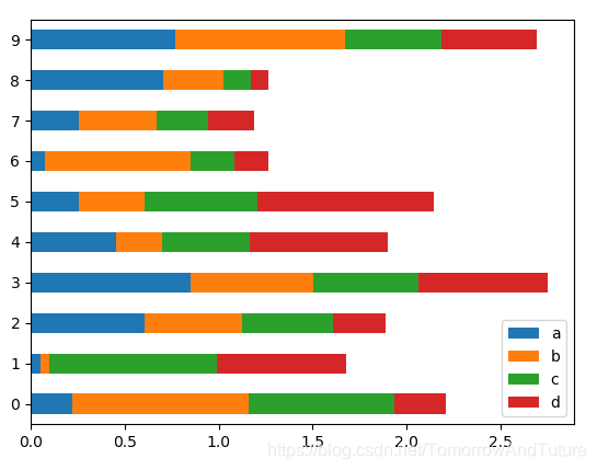
>>> df = pd.DataFrame(np.random.rand(10,4),columns=['a','b','c','d'])
>>> df
          a         b         c         d
0  0.223895  0.934126  0.776715  0.272412
1  0.054357  0.044082  0.890138  0.692204
2  0.603401  0.522171  0.483764  0.277524
3  0.851305  0.649713  0.559654  0.691692
4  0.453478  0.247265  0.464155  0.733652
5  0.257328  0.348949  0.598477  0.938713
6  0.073403  0.776095  0.235249  0.177406
7  0.255504  0.414014  0.275384  0.243649
8  0.704180  0.320717  0.143664  0.097838
9  0.770821  0.903387  0.507908  0.510510
>>> df.plot.bar()
<matplotlib.axes._subplots.AxesSubplot object at 0x0000000019689438>
>>> df.plot.bar(stacked=True)
<matplotlib.axes._subplots.AxesSubplot object at 0x0000000018120B00>
>>> df.plot.barh(stacked=True)
<matplotlib.axes._subplots.AxesSubplot object at 0x00000000180BE320>
>>> plt.show() 

>>> df = pd.DataFrame(np.random.rand(10, 5), columns=['A', 'B', 'C', 'D', 'E'])
>>> df
          A         B         C         D         E
0  0.128757  0.113134  0.960562  0.232801  0.015381
1  0.832828  0.826641  0.668275  0.411818  0.100598
2  0.896566  0.870508  0.649730  0.272994  0.193057
3  0.993245  0.795654  0.401693  0.062322  0.181763
4  0.907362  0.512175  0.226137  0.362590  0.919171
5  0.189321  0.117297  0.863777  0.957350  0.680298
6  0.377515  0.003974  0.769770  0.483371  0.477716
7  0.857534  0.307702  0.466231  0.141965  0.804760
8  0.449878  0.676380  0.666671  0.960456  0.082041
9  0.841580  0.872631  0.127302  0.386110  0.163839
>>> df.plot.box()
<matplotlib.axes._subplots.AxesSubplot object at 0x0000000018165780>
>>> df.plot.area()
<matplotlib.axes._subplots.AxesSubplot object at 0x0000000019BA3FD0>
>>> df.plot.scatter(x='A', y='B')
<matplotlib.axes._subplots.AxesSubplot object at 0x00000000141EB358>
>>> plt.show() 


>>> df = pd.DataFrame(3 * np.random.rand(4), index=['a', 'b', 'c', 'd'], columns=['x'])
>>> df
          x
a  0.842394
b  0.773727
c  1.644047
d  2.104003
>>> df.plot.pie(subplots=True)
array([<matplotlib.axes._subplots.AxesSubplot object at 0x0000000019549240>],
      dtype=object)
>>> plt.show() 
IO工具
>>> import numpy as np
>>> import pandas as pd
>>> df = pd.read_csv('temp.csv')
>>> df
   S.No    Name  Age       City  Salary
0     1     Tom   28    Toronto   20000
1     2     Lee   32   HongKong    3000
2     3  Steven   43   Bay area    8300
3     4     Ram   38  Hyderabad    3900
>>> df = pd.read_csv('temp.csv', index_col=['S.No'])
>>> df
        Name  Age       City  Salary
S.No
1        Tom   28    Toronto   20000
2        Lee   32   HongKong    3000
3     Steven   43   Bay area    8300
4        Ram   38  Hyderabad    3900
>>> pd.read_csv('temp.csv', dtype={'Salary':np.float64})
   S.No    Name  Age       City   Salary
0     1     Tom   28    Toronto  20000.0
1     2     Lee   32   HongKong   3000.0
2     3  Steven   43   Bay area   8300.0
3     4     Ram   38  Hyderabad   3900.0
>>> pd.read_csv('temp.csv', names=['a', 'b', 'c', 'd', 'e'])
      a       b    c          d       e
0  S.No    Name  Age       City  Salary
1     1     Tom   28    Toronto   20000
2     2     Lee   32   HongKong    3000
3     3  Steven   43   Bay area    8300
4     4     Ram   38  Hyderabad    3900
>>> pd.read_csv('temp.csv', names=['a', 'b', 'c', 'd', 'e'], header=0)
   a       b   c          d      e
0  1     Tom  28    Toronto  20000
1  2     Lee  32   HongKong   3000
2  3  Steven  43   Bay area   8300
3  4     Ram  38  Hyderabad   3900
>>> pd.read_csv('temp.csv', skiprows=2)
   2     Lee  32   HongKong  3000
0  3  Steven  43   Bay area  8300
1 4 Ram 38 Hyderabad 3900 
稀疏数据
>>> ts = pd.Series(np.random.randn(10))
>>> ts[2:-2] = np.nan
>>> sts = ts.to_sparse()
>>> sts
0   -0.585138
1    0.893830
2         NaN
3         NaN
4         NaN
5         NaN
6         NaN
7         NaN
8    0.135530
9   -1.513085
dtype: float64
BlockIndex
Block locations: array([0, 8])
Block lengths: array([2, 2])
>>> ts
0   -0.585138
1    0.893830
2         NaN
3         NaN
4         NaN
5         NaN
6         NaN
7         NaN
8    0.135530
9   -1.513085
dtype: float64
>>> sts.to_dense()
0   -0.585138
1    0.893830
2         NaN
3         NaN
4         NaN
5         NaN
6         NaN
7         NaN
8    0.135530
9   -1.513085
dtype: float64
>>> sts
0   -0.585138
1    0.893830
2         NaN
3         NaN
4         NaN
5         NaN
6         NaN
7         NaN
8    0.135530
9   -1.513085
dtype: float64
BlockIndex
Block locations: array([0, 8])
Block lengths: array([2, 2])
>>> sts.density
0.4