1.导入波士顿房价数据
![[外链图片转存失败,源站可能有防盗链机制,建议将图片保存下来直接上传(img-IjpXtJVg-1596197641549)(attachment:image.png)]](https://img-blog.csdnimg.cn/20200731201423397.png?x-oss-process=image/watermark,type_ZmFuZ3poZW5naGVpdGk,shadow_10,text_aHR0cHM6Ly9ibG9nLmNzZG4ubmV0L2NoYWlyb24=,size_16,color_FFFFFF,t_70)
import numpy as np
import pandas as pd

data=pd.read_csv("data/boston.csv")
data
| CRIM | ZN | INDUS | CHAS | NOX | RM | AGE | DIS | RAD | TAX | PTRATIO | B | LSTAT | MEDV | |
|---|---|---|---|---|---|---|---|---|---|---|---|---|---|---|
| 0 | 0.00632 | 18.0 | 2.31 | 0 | 0.538 | 6.575 | 65.2 | 4.0900 | 1 | 296 | 15.3 | 396.90 | 4.98 | 24.0 |
| 1 | 0.02731 | 0.0 | 7.07 | 0 | 0.469 | 6.421 | 78.9 | 4.9671 | 2 | 242 | 17.8 | 396.90 | 9.14 | 21.6 |
| 2 | 0.02729 | 0.0 | 7.07 | 0 | 0.469 | 7.185 | 61.1 | 4.9671 | 2 | 242 | 17.8 | 392.83 | 4.03 | 34.7 |
| 3 | 0.03237 | 0.0 | 2.18 | 0 | 0.458 | 6.998 | 45.8 | 6.0622 | 3 | 222 | 18.7 | 394.63 | 2.94 | 33.4 |
| 4 | 0.06905 | 0.0 | 2.18 | 0 | 0.458 | 7.147 | 54.2 | 6.0622 | 3 | 222 | 18.7 | 396.90 | 5.33 | 36.2 |
| ... | ... | ... | ... | ... | ... | ... | ... | ... | ... | ... | ... | ... | ... | ... |
| 501 | 0.06263 | 0.0 | 11.93 | 0 | 0.573 | 6.593 | 69.1 | 2.4786 | 1 | 273 | 21.0 | 391.99 | 9.67 | 22.4 |
| 502 | 0.04527 | 0.0 | 11.93 | 0 | 0.573 | 6.120 | 76.7 | 2.2875 | 1 | 273 | 21.0 | 396.90 | 9.08 | 20.6 |
| 503 | 0.06076 | 0.0 | 11.93 | 0 | 0.573 | 6.976 | 91.0 | 2.1675 | 1 | 273 | 21.0 | 396.90 | 5.64 | 23.9 |
| 504 | 0.10959 | 0.0 | 11.93 | 0 | 0.573 | 6.794 | 89.3 | 2.3889 | 1 | 273 | 21.0 | 393.45 | 6.48 | 22.0 |
| 505 | 0.04741 | 0.0 | 11.93 | 0 | 0.573 | 6.030 | 80.8 | 2.5050 | 1 | 273 | 21.0 | 396.90 | 7.88 | 11.9 |
506 rows × 14 columns
#查看数据的基本信息。同时也可以查看是否有缺失值
data.info()
#查看是否有重复值
data.duplicated().any()
<class 'pandas.core.frame.DataFrame'>
RangeIndex: 506 entries, 0 to 505
Data columns (total 14 columns):
 #   Column   Non-Null Count  Dtype
---  ------   --------------  -----
 0   CRIM     506 non-null    float64
 1   ZN       506 non-null    float64
 2   INDUS    506 non-null    float64
 3   CHAS     506 non-null    int64
 4   NOX      506 non-null    float64
 5   RM       506 non-null    float64
 6   AGE      506 non-null    float64
 7   DIS      506 non-null    float64
 8   RAD      506 non-null    int64
 9   TAX      506 non-null    int64
 10  PTRATIO  506 non-null    float64
 11  B        506 non-null    float64
 12  LSTAT    506 non-null    float64
 13  MEDV     506 non-null    float64
dtypes: float64(11), int64(3)
memory usage: 55.5 KB


False
2. 实现线性回归(最小二乘法)
class LinearRegression:
    """最小二乘法实现"""
    def fit(self,X,y):
        #注意:X必须是完整的矩阵,通过拷贝X,避免X只是数组对象的一部分(进行了切片)
        X=np.asmatrix(X.copy())
        #y是一维,可以不用进行拷贝,因为进行矩阵运算,必须转化为二维矩阵
        y=np.asmatrix(y).reshape(-1,1)
        #通过最小二乘公式,求解出最佳的权重值
        self.w_=(X.T*X).I*X.T*y

    def predict(self,X):

        X=np.asmatrix(X.copy())
        result=X*self.w_
        #将矩阵转化为数组,使用ravel()进行扁平化处理
        return np.array(result).ravel()
3. 数据切分,进行预测
3.1 不考虑截距
t=data.sample(len(data),random_state=666)
train_X=t.iloc[:400,:-1]
train_y=t.iloc[:400,-1]
test_X=t.iloc[400:,:-1]
test_y=t.iloc[400:,-1]

my_reg=LinearRegression()
my_reg.fit(train_X,train_y)
result=my_reg.predict(test_X)
#result
display(np.mean((result-test_y)**2))
#查看权重值
display(my_reg.w_)
18.595095881220296


matrix([[-2.13527048e-01],
        [ 4.64325786e-02],
        [-4.40798167e-02],
        [ 3.94148352e+00],
        [-2.43031921e+00],
        [ 5.60499592e+00],
        [-3.53223856e-03],
        [-9.53062020e-01],
        [ 2.00556858e-01],
        [-9.05450000e-03],
        [-2.68508504e-01],
        [ 1.53991325e-02],
        [-4.94776734e-01]])
3.2 考虑截距:
增加一列,该列的所有值为1
t=data.sample(len(data),random_state=666)
#t["Intercept"]=1
#t
#按照习惯截距作为w0,为之配上一个x0,放在最前面
new_columns=t.columns.insert(0,"Intercept")
#t=t.reindex(columns=new_columns)
#t["Intercept"]=1
#重新安排列的序列,如果值为空,使用fill_value参数填充
t=t.reindex(columns=new_columns,fill_value=1)


train_X=t.iloc[:400,:-1]
train_y=t.iloc[:400,-1]
test_X=t.iloc[400:,:-1]
test_y=t.iloc[400:,-1]

my_reg2=LinearRegression()
my_reg2.fit(train_X,train_y)
result2=my_reg2.predict(test_X)
#result
display(np.mean((result2-test_y)**2))
#查看权重值
display(my_reg2.w_)
18.706069253903184


matrix([[ 3.83679438e+01],
        [-1.70796105e-02],
        [ 4.08402871e-02],
        [-7.84161928e-03],
        [ 3.94149503e+00],
        [-1.85251673e+01],
        [ 3.46054943e+00],
        [ 1.54653190e-03],
        [-1.46077566e+00],
        [ 2.87513235e-01],
        [-1.24453964e-02],
        [-8.57033425e-01],
        [ 9.42230048e-03],
        [-6.08173883e-01]])
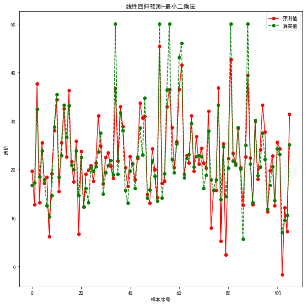
4. 可视化展示
import matplotlib as mpl
import matplotlib.pyplot as plt

mpl.rcParams["font.family"]="SimHei"
mpl.rcParams["axes.unicode_minus"]=False

plt.figure(figsize=(10,10))
#绘制预测值
plt.plot(result2,"ro-",label="预测值")
#绘制真实值
plt.plot(test_y.values,"go--",label="真实值")
plt.title("线性回归预测-最小二乘法")
plt.xlabel("样本序号")
plt.ylabel("房价")
plt.legend()
<matplotlib.legend.Legend at 0x20f9d9defc8>