目录--------------------------------持续更新
对应点相乘,
x.mul(y) ,即点乘操作,点乘不求和操作,又可以叫作Hadamard product;点乘再求和,即为卷积
>>> a = torch.Tensor([[1,2], [3,4], [5, 6]])
>>> a
tensor([[1., 2.],
        [3., 4.],
        [5., 6.]])
>>> a.mul(a)
tensor([[ 1.,  4.],
        [ 9., 16.],
        [25., 36.]])

# a*a等价于a.mul(a)
矩阵相乘,
x.mm(y) , 矩阵大小需满足: (i, n)x(n, j)
>>> a
tensor([[1., 2.],
        [3., 4.],
        [5., 6.]])
>>> b = a.t()  # 转置
>>> b
tensor([[1., 3., 5.],
        [2., 4., 6.]])

>>> a.mm(b)
tensor([[ 5., 11., 17.],
        [11., 25., 39.],
        [17., 39., 61.]])
矩阵相乘(维度不同,可广播)
torch.matmul()
torch.matmul(input, other, out=None) → Tensor
#两个张量的矩阵乘积。行为取决于张量的维数,如下所示:
#1. 如果两个张量都是一维的,则返回点积(标量)。
>>> # vector x vector
>>> tensor1 = torch.randn(3)
>>> tensor2 = torch.randn(3)
>>> torch.matmul(tensor1, tensor2).size()
torch.Size([])
#2. 如果两个参数都是二维的,则返回矩阵矩阵乘积。
# matrix x matrix
>>> tensor1 = torch.randn(3, 4)
>>> tensor2 = torch.randn(4, 5)
>>> torch.matmul(tensor1, tensor2).size()
torch.Size([3, 5])
#3. 如果第一个参数是一维的,而第二个参数是二维的,则为了矩阵乘法,会将1附加到其维数上。矩阵相乘后,将删除前置尺寸。
# 也就是让tensor2变成矩阵表示,1x3的矩阵和 3x4的矩阵,得到1x4的矩阵,然后删除1
>>> tensor1 = torch.randn(3, 4)
>>> tensor2 = torch.randn(3)
>>> torch.matmul(tensor2, tensor1).size()
torch.Size([4])
#4. 如果第一个参数为二维,第二个参数为一维,则返回矩阵向量乘积。
# matrix x vector
>>> tensor1 = torch.randn(3, 4)
>>> tensor2 = torch.randn(4)
>>> torch.matmul(tensor1, tensor2).size()
torch.Size([3])
#5. 如果两个自变量至少为一维且至少一个自变量为N维(其中N> 2),则返回批处理矩阵乘法。如果第一个参数是一维的,则在其维数之前添加一个1,以实现批量矩阵乘法并在其后删除。如果第二个参数为一维,则将1附加到其维上,以实现成批矩阵倍数的目的,然后将其删除。非矩阵(即批量)维度可以被广播(因此必须是可广播的)。例如,如果input为(jx1xnxm)张量,而other为(k×m×p)张量,out将是(j×k×n×p)张量。
>>> # batched matrix x broadcasted vector
>>> tensor1 = torch.randn(10, 3, 4)
>>> tensor2 = torch.randn(4)
>>> torch.matmul(tensor1, tensor2).size()
torch.Size([10, 3])
>>> # batched matrix x batched matrix
>>> tensor1 = torch.randn(10, 3, 4)
>>> tensor2 = torch.randn(10, 4, 5)
>>> torch.matmul(tensor1, tensor2).size()
torch.Size([10, 3, 5])
>>> # batched matrix x broadcasted matrix
>>> tensor1 = torch.randn(10, 3, 4)
>>> tensor2 = torch.randn(4, 5)
>>> torch.matmul(tensor1, tensor2).size()
torch.Size([10, 3, 5])
>>> tensor1 = torch.randn(10, 1, 3, 4)
>>> tensor2 = torch.randn(2, 4, 5)
>>> torch.matmul(tensor1, tensor2).size()
torch.Size([10, 2, 3, 5])
上采样——nn.Upsample
import torch
from torch import nn
input = torch.arange(1, 5, dtype=torch.float32).view(1, 1, 2, 2)
input
tensor([[[[1., 2.],
          [3., 4.]]]])


m = nn.Upsample(scale_factor=2, mode='nearest')
m(input)
tensor([[[[1., 1., 2., 2.],
          [1., 1., 2., 2.],
          [3., 3., 4., 4.],
          [3., 3., 4., 4.]]]])


m = nn.Upsample(scale_factor=2, mode='bilinear',align_corners=False)
m(input)
tensor([[[[1.0000, 1.2500, 1.7500, 2.0000],
          [1.5000, 1.7500, 2.2500, 2.5000],
          [2.5000, 2.7500, 3.2500, 3.5000],
          [3.0000, 3.2500, 3.7500, 4.0000]]]])


m = nn.Upsample(scale_factor=2, mode='bilinear',align_corners=True)
m(input)
tensor([[[[1.0000, 1.3333, 1.6667, 2.0000],
          [1.6667, 2.0000, 2.3333, 2.6667],
          [2.3333, 2.6667, 3.0000, 3.3333],
          [3.0000, 3.3333, 3.6667, 4.0000]]]])


m = nn.Upsample(size=(3,5), mode='bilinear',align_corners=True)
m(input)
tensor([[[[1.0000, 1.2500, 1.5000, 1.7500, 2.0000],
          [2.0000, 2.2500, 2.5000, 2.7500, 3.0000],
          [3.0000, 3.2500, 3.5000, 3.7500, 4.0000]]]])
损失函数
- nn.L1Loss
取预测值和真实值的绝对误差的平均数。 - nn.SmoothL1Loss
也叫作 Huber Loss,误差在 (-1,1) 上是平方损失,其他情况是 L1 损失。 - nn.MSELoss
即平方损失函数,预测值和真实值之间的平方和的平均数 - nn.BCELoss
BinaryCrossEntropy二值交叉熵损失函数,用于二分类

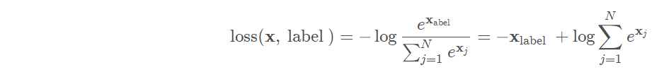
- nn.CrossEntropyLoss
交叉熵损失函数。
- nn.functional.nll_loss
负对数似然损失函数(Negative Log Likelihood)

- nn.NLLLoss2d
扩展维度的nll_loss
import torch
from torch.autograd import Variable
import torch.nn as nn
import torch.nn.functional as F
sample = Variable(torch.ones(2,2))
target = Variable (torch.zeros(2,2))

# nn.L1Loss
criterion = nn.L1Loss()
loss = criterion(sample, target)
print('nn.L1Loss: ', loss)
# nn.L1Loss:  tensor(1.)

# nn.SmoothL1Loss
criterion = nn.SmoothL1Loss()
loss = criterion(sample, target)
print('nn.SmoothL1Loss: ', loss)
# nn.SmoothL1Loss:  tensor(0.5000)

# nn.MSELoss
criterion = nn.MSELoss()
loss = criterion(sample, target)
print('nn.MSELoss: ', loss)
# nn.MSELoss:  tensor(1.)

# nn.BCELoss
criterion = nn.BCELoss()
loss = criterion(sample, target)
print('nn.BCELoss: ', loss)
# nn.BCELoss:  tensor(27.6310)

# nn.CrossEntropyLoss
criterion = nn.CrossEntropyLoss()
loss = criterion(sample, target)
print(loss)
# 报错 target需要scalar type Long

# nn.functional.nll_loss
criterion = F.nll_loss()
loss = criterion(sample, target)
print(loss)
loss=F.nll_loss(sample,target)
# 报错 target需要scalar type Long

# nn.NLLLoss2d
criterion = nn.NLLLoss2d()
loss = criterion(sample, target)
print(loss)
# 报错 target需要scalar type Long
tensor选择某维度的几个数据
torch.index_select(input, dim, index, out=None)
沿着指定维度对输入进行切片,取index中指定的相应项,返回一个新的张量,返回的张量与原始的张量有相同的维度。返回张量不与原始张量共享内存中的空间。
参数:
input(Tensor) – 输入张量
dim(int) – 索引的维度
index(LongTensor) – 包含索引下标的一维张量
out(Tensor, 可选) – 目标张量
>>> x = torch.randn(3, 4)
>>> x
tensor([[-1.0190, -0.7541,  2.1090, -0.9576],
        [-1.4745,  0.1462, -2.2930, -0.9130],
        [ 0.7339, -2.0842, -0.9208, -0.5618]])
>>> indices = torch.LongTensor([0, 2])
>>> torch.index_select(x, 0, indices)
tensor([[-1.0190, -0.7541,  2.1090, -0.9576],
        [ 0.7339, -2.0842, -0.9208, -0.5618]])
>>> torch.index_select(x, 1, indices)
tensor([[-1.0190,  2.1090],
        [-1.4745, -2.2930],
        [ 0.7339, -0.9208]])
索引、切片、连接、变异操作
https://blog.csdn.net/gyt15663668337/article/details/91345951
扩大压缩张量
x = torch.Tensor([[1], [2], [3]])
x.size()
torch.Size([3, 1])
x.expand(3, 4)
1 1 1 1
2 2 2 2
3 3 3 3
[torch.FloatTensor of size 3x4]

x = torch.zeros(2, 1, 2, 1, 2)
x.size()
torch.Size([2, 1, 2, 1, 2])
y = torch.squeeze(x)
y.size()
torch.Size([2, 2, 2])
y = torch.squeeze(x, 0)
y.size()
torch.Size([2, 1, 2, 1, 2])
y = torch.squeeze(x, 1)
y.size()
torch.Size([2, 2, 1, 2])
拼接、维度扩展、压缩、转置、重复……
全局平均池化GAP
torch.nn.functional.adaptive_avg_pool2d(output, (1, 1))