0.导入相关包：

import matplotlib.pyplot as plt
import numpy as np

1.假设有如下样本点：

#使用随机数产生样本点
x=[1,2,3,4,5,6,7,8,9,10]
y=[2,-25,16,3,35,6,91,-39,20,0]
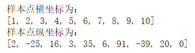
print("样本点横坐标为：")
print(x)
print("样本点纵坐标为：")
print(y)

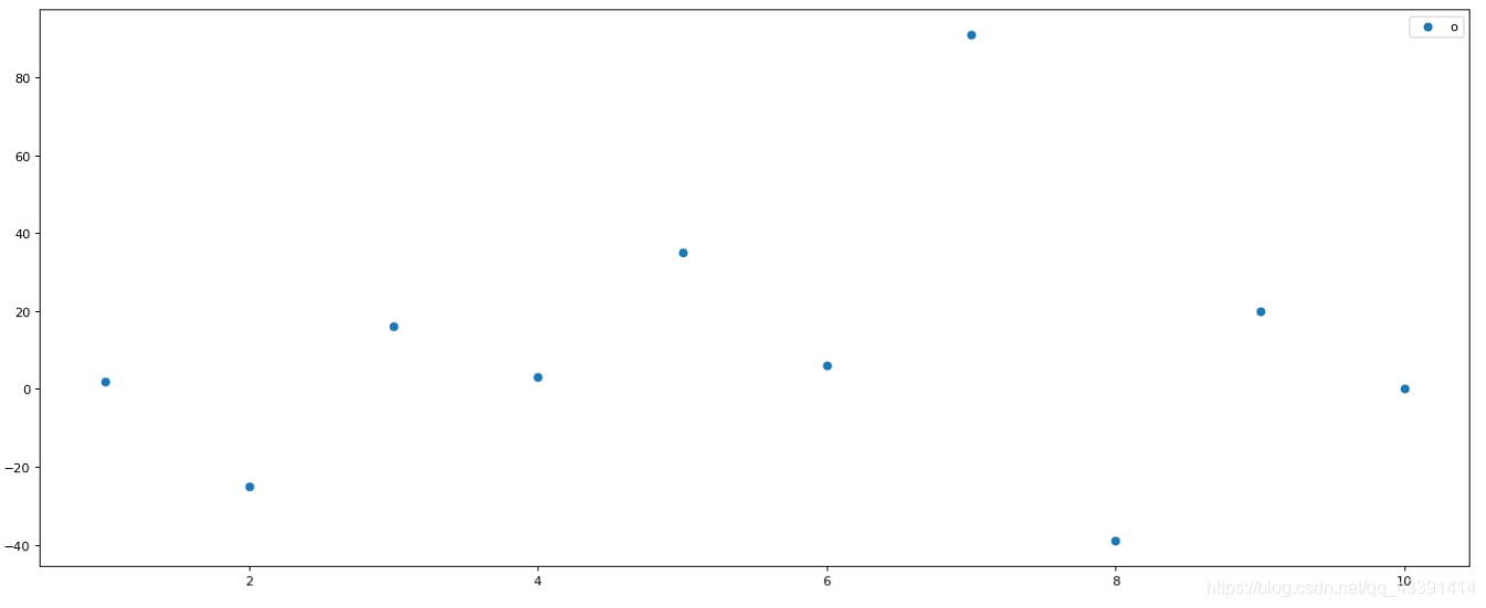
绘制成散点图就是这样：

2.我们利用numpy来拟合这些样本点，本文中我们将函数拟合成多项式函数。（核心步骤）

#使用numpy中的多项式拟合来拟合样本服从的函数。
#下面分别假设多项式最高次数为4，7，8。从而进行对比拟合效果。
degree=[4,7,8]
#每一个最高次数degree对应一个多项式函数，因此创建一个函数数组。
f=[]
for i in range(3):
    #拟合
    model=np.polyfit(x,y,degree[i])
    #通过拟合的模型获得这个多项式函数np.poly1d(model)。
    f.append(np.poly1d(model))
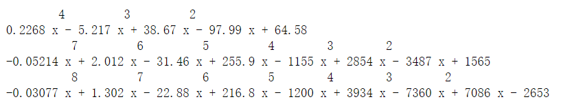
    #打印这个函数
    print(f[i])

结果如下：

3.绘制图表，查看拟合情况。

#开始绘制。
colors=["r","g","orange","purple","pink"]
#生成1000个点在区间[1,10]，利用拟合结果f(x)得到y。绘制折线图，由于密密麻麻，所以看起来就像函数图像了。
testx=np.linspace(1,10,1000)
plt.figure(figsize=(20,8),dpi=80)
for i in range(3):
    plt.plot(testx,f[i](testx),label=degree[i],color=colors[i])

plt.scatter(x,y,label="o")    
plt.legend()
plt.show()

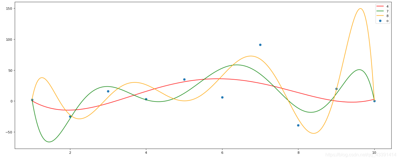
结论

多项式次数越高，拟合得越好。