数据集data介绍
MNIST数据集(Mixed National Institute of Standards and Technology database)是美国国家标准与技术研究院收集整理的大型手写数字数据库,包含60,000个示例的训练集以及10,000个示例的测试集。每张图片的长度和宽度都是28. y值是0-9,代表10个数字。
Load data by using TF
(trainX,trainY), (testX,testY) = tf.keras.datasets.mnist.load_data()
已知y的取值是0-9,那么x则是图像显示0-9. 把前几张图片显示出来。
# 把X的部分图片表现出来
for i in range(9):
	# define subplot
	plt.subplot(331+i)
	# plot raw pixel data
	plt.imshow(trainX[i], cmap=plt.get_cmap('gray'))
# show the figure
plt.show()

(1)Data Preprocessing
首先,我们需要从train data 取20%的作为valid data。这里可以使用train_test_split()函数来分离出20%data 作为valid data
from sklearn.model_selection import train_test_split
X_train, X_valid, Y_train, Y_valid = train_test_split(trainX,trainY,test_size=0.2)
然后,需要把图片的28*28data,进行扁平化。变成784。然后再进行normalized化,除最大值255,使得数值映射到0-1内。
对feature set X进行处理(扁平化+normalized)
#对于X_train,X_valid,X_test扁平化再normalize
X_train_reshape = tf.cast(X_train.reshape((X_train.shape[0],-1))/255.0,dtype='float32')
X_valid_reshape = tf.cast(X_valid.reshape((X_valid.shape[0],-1))/255.0,dtype='float32')
X_test_reshape = tf.cast(X_test.reshape((X_test.shape[0],-1))/255.0,dtype='float32')
对y值进行one hot 处理
one hot处理,比如y=1,则转换为y=[0,1,0,0,0,0,0,0,0,0],即array位置对应着相应的数字。
# one hot encode target values
y_train_encode = tf.one_hot(y_train,depth = 10)
y_valid_encode = tf.one_hot(y_valid,depth = 10)
y_test_encode = tf.one_hot(y_test,depth = 10)
(2)模型的设置
设置两层的layers里的networks。 详细的介绍:
在这次神经网络中,input的神经元为784个,hidden 的神经元为128个,output的神经元为10个。用来分类。公式为
h 1 = R e L U ( X W 1 + b 1 ) h_1 = ReLU(XW_1 + b_1) h1=ReLU(XW1+b1) Y = h 1 W 2 + b 2 Y = h_1W_2 + b_2 Y=h1W2+b2
第一层是,input是X_train_reshape的shape为 (48000,784)。W1的shape为(784,128),b1的shape为(1,128). 经过W1和b1的转换,变成128个神经元,再经过激活函数relu来输出为h。这是第一层。
下一层的参数W2的shape为(128,10),b2的shape为(1,10),经过W2,和b2的转换,变成10个神经元,再经过sigmoid激活函数输出每个类的概率值。取其中最大的概率的那个类作为pred值。
参数的初始值设置
理解模型所需的参数之后,开始定义初始值的参数 W1, W2, b1, b2。这里我们定义W1和W2的初始值为0.01,b1,b2初始值定义为0
#W_1的值全部为 0.01 , size 为784*128
W_1 = tf.Variable(tf.ones(shape=[784,128])/100)
#b_1的值全部为0,size为1*128
b1 = tf.Variable(tf.zeros(shape=[128]))

#W_2的值全部为 0.01 , size 为128*10
W_2 = tf.Variable(tf.ones(shape=[128,10])/100)
#b_2的值全部为0,size为1*10
b2 = tf.Variable(tf.zeros(shape=[10]))
定义模型的函数
def feedforward(X):
  '''
  Implement the feed forward step for given X
  hidden_out = ReLU(X*W1 + b1)
  output = hidden_output * W2 + b2
  '''
  #matmul就是普通的矩阵相乘 需要里面的维度相同,比如 (3,2)*(2,3)=(3,3)
    hidden_in = tf.add(tf.matmul(X,W1), b1)      #公式X*W1 + b1
    hidden_out = tf.nn.relu(hidden_in)           #激活函数出来
    output = tf.add(tf.matmul(hidden_out,W2),b2) #hidden_out * W2 + b2
    return output
开始训练模型Using TF
#定义优化器
optimizer = tf.keras.optimizers.SGD(learning_rate=0.5)
设置
def one_step_train(x,y,optim, W_1 = W_1, b1 = b1, W_2 = W_2, b2 = b2):
  with tf.GradientTape() as tape:
    #求的 y_pred = logit--还没使用softmax函数计算概率,下一步会用tf里面内置函数计算
    train_logit = feedforward (x)
    #计算loss function --cross entropy【y是one hot后的实际值】
    train_cross_en = tf.nn.softmax_cross_entropy_with_logits(labels = y,
                                                             logits = train_logit)
    train_loss = tf.reduce_mean(train_cross_en)  #对loss取平均值

  #对W1,W2,b1,b2 计算梯度
  grads = tape.gradient(train_loss,[W_1,b1,W_2,b2])
  optim.apply_gradients(zip(grads,[W_1,b1,W_2,b2]))  #更新所有的参数W1,W2,b1,b2
  return train_loss
解释tf内置函数
- tf.nn.softmax() 函数
#随机设置两个samples 值对应的y labels和x输出的logits值
labels = [[0,0,1,0,0,0,0,0,0,0], [0,0,0,0,1,0,0,0,0,0]]
logits = [[0.1,0.2,0.3,0.5,0.2,0.3,0.4,0.5,0.2,0.1], [0.1,0.2,0.3,0.5,0.2,0.3,0.4,0.5,0.2,0.1]]
计算这两个samples的里面每个的softmax值,shape为(2,10)
logit_scaled = tf.nn.softmax(logits)
print(logit_scaled)

计算loss值
result = tf.nn.softmax_cross_entropy_with_logits(labels = labels, logits = logits)
print(result)

这里这两个值代表这两个sample的loss值,后面会算一个mean值作为总loss值。使用tf.reduce_mean()函数
train_loss = tf.reduce_mean(result)
所以把这些总结在一起,便是one step train 函数
def one_step_train(x,y,optim, W_1 = W1, b_1 = b1, W_2 = W2, b_2 = b2):
  with tf.GradientTape() as tape:
    #求的 y_pred = logit--还没使用softmax函数计算概率,下一步会用tf里面内置函数计算
    train_logit = feedforward (x)
    #计算loss function --cross entropy【y是one hot后的实际值】
    train_cross_en = tf.nn.softmax_cross_entropy_with_logits(labels = y,
                                                             logits = train_logit)
    train_loss = tf.reduce_mean(train_cross_en)  #对loss取平均值最为最后的train_loss值

  #对W1,W2,b1,b2 计算梯度
  grads = tape.gradient(train_loss,[W_1,b_1,W_2,b_2])
  optim.apply_gradients(zip(grads,[W_1,b_1,W_2,b_2]))
  return train_loss
(3)模型的迭代
#迭代的次数 1000次
iterations = 1000
#store the training losses
train_loss_ls = []
#store the validation losses
valid_loss_ls = []
for i in range(iterations):
train_loss = one_step_train(X_train_reshape,y_train_encode,optim = optimizer)
valid_logits = feedforward(X_valid_reshape)
valid_cross_en = tf.nn.softmax_cross_entropy_with_logits(labels = y_valid_encode,
logits = valid_logits)
valid_loss = tf.reduce_mean(valid_cross_en)
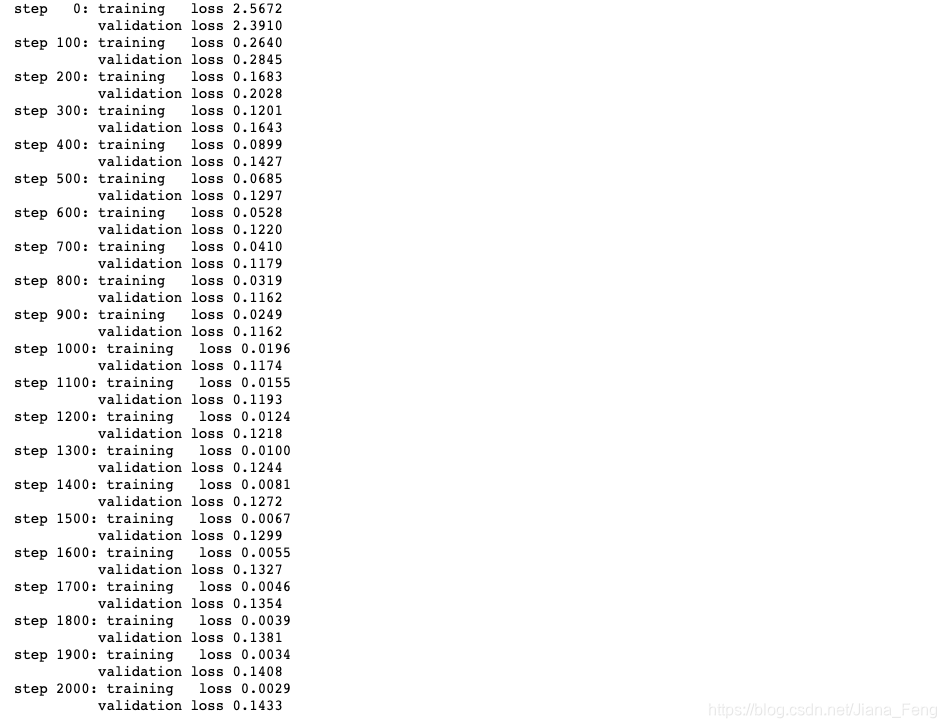
if i % 100 == 0:
print('step {0:3d}: training loss {1:.4f} \n\t validation loss {2:.4f}'.format(i, train_loss,valid_loss))
train_loss_ls.append(train_loss)
valid_loss_ls.append(valid_loss)

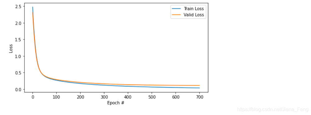
(4)把train loss和valid loss 可视化
fig, ax = plt.subplots(figsize=(8,4))
ax.plot(train_loss_ls, label='Train Loss')
ax.plot(valid_loss_ls, label='Valid Loss')
ax.set_xlabel("Epoch #")
ax.set_ylabel("Loss")
ax.legend();

(5)模型的比较
改一下模型的optimizer优化器和参数,看看哪个模型的效果更好
- Option A: tf.keras.optimizers.SGD with learning rate = 0.5
- Option B: tf.keras.optimizers.SGD with learning rate = 0.001
- Option C: tf.keras.optimizers.Adam with learning rate = 0.001
Option A就是上面我们已经实践过的模型。接下来是实践模型B和模型C
实践模型B
tf.keras.optimizers.SGD with learning rate = 0.001
- 初始化参数
W_1 = tf.Variable(tf.ones(shape=[784,128])/100)
b_1 = tf.Variable(tf.zeros(shape= [128]))
W_2 = tf.Variable(tf.ones(shape= [128,10])/100)
b_2 = tf.Variable(tf.zeros(shape= [10]))
- 设置优化器的参数
optim_B = tf.keras.optimizers.SGD(learning_rate = 0.001)
- 开始训练和迭代模型
#迭代数为2000
iterations = 2001
#store the training losses
train_loss_ls_B = []
#store the validation losses
valid_loss_ls_B = []
#书写训练模型的迭代
for i in range(iterations):
	#利用上次的one_step_train来计算train的 loss
	train_loss = one_step_train(X_train_reshape,y_train_encode, optim = optim_B)
	#开始一步一步写valid的loss,因为需要把上一步更新过的参数来计算valid loss
	valid_logits = feedforward(X_valid_reshape)
	#计算所有samlpes的loss值
	valid_cross_en = tf.nn.softmax_cross_entropy_with_logits(labels = y_valid_encode,logits = valid_logits)
	#计算平均loss值作为valid_loss
	valid_loss = tf.reduce_mean(valid_cross_en)
	if ii % 100 == 0:
		print('step {0:3d}: training   loss {1:.4f} \n\t  validation loss {2:.4f}'.format(i, train_loss,valid_loss))
	train_loss_ls_B.append(train_loss)
	valid_loss_ls_B.append(valid_loss)

实践模型C
tf.keras.optimizers.Adam with learning rate = 0.001
- 初始化参数
W_1 = tf.Variable(tf.ones(shape=[784,128])/100)
b_1 = tf.Variable(tf.zeros(shape= [128]))
W_2 = tf.Variable(tf.ones(shape= [128,10])/100)
b_2 = tf.Variable(tf.zeros(shape= [10]))
- 设置优化器的参数
optim_C = tf.optimizers.Adam(learning_rate = 0.001)
- 开始训练和迭代模型
#迭代数为2000
iterations = 2001
#store the training losses
train_loss_ls_C = []
#store the validation losses
valid_loss_ls_C = []
#书写训练模型的迭代
for i in range(iterations):
	#利用上次的one_step_train来计算train的 loss
	train_loss = one_step_train(X_train_reshape,y_train_encode, optim = optim_C)
	#开始一步一步写valid的loss,因为需要把上一步更新过的参数来计算valid loss
	valid_logits = feedforward(X_valid_reshape)
	#计算所有samlpes的loss值
	valid_cross_en = tf.nn.softmax_cross_entropy_with_logits(labels = y_valid_encode,logits = valid_logits)
	#计算平均loss值作为valid_loss
	valid_loss = tf.reduce_mean(valid_cross_en)
	if ii % 100 == 0:
		print('step {0:3d}: training   loss {1:.4f} \n\t  validation loss {2:.4f}'.format(i, train_loss,valid_loss))
	train_loss_ls_C.append(train_loss)
	valid_loss_ls_C.append(valid_loss)

总结
第一个模型A,可以看出train loss在摇摆,时大时小,证明了模型A并不是很适合来训练data。
第二个模型B,loss反而上升来,并没有对模型进行改进。
第三模型C,可以明显看到loss下降。所以模型C是最适合的。
(6)参数W初始值的比较
由上面可知,Adam模型是最适合的。现在来比较初始值W选取对loss的影响。
- Option A: 初始值W设置为0.001
- Option B: 用标准正太分布来随意设置初始值W (mean = 0, sd = 1)
- Option C: 用正太分布来随意设置初始值 W (mean=0,sd = 0.1)
Option A:初始值W设置为0.001
#初始值W设置为0.001
W_1 = tf.Variable(tf.ones(shape=[784,128])/1000)
b_1 = tf.Variable(tf.zeros(shape= [128]))
W_2 = tf.Variable(tf.ones(shape= [128,10])/1000)
b_2 = tf.Variable(tf.zeros(shape= [10]))
#选择Adam优化器
optim_C = tf.optimizers.Adam(learning_rate = 0.001)

iterations = 2001
#store the training losses
train_loss_ls_C = []
#store the validation losses
valid_loss_ls_C = []
for ii in range(iterations):
    train_loss = one_step_train(X_train_reshape,y_train_encode,optim = optim_C)
    #after update the weight check the validation result
    valid_logits = feedforward(X_valid_reshape)
    valid_cross_en = tf.nn.softmax_cross_entropy_with_logits(labels = y_valid_encode,
                                                             logits = valid_logits)
    #compute validation loss
    valid_loss = tf.reduce_mean(valid_cross_en)
    # Printing out the training progress per 100 epochs
    if ii % 100 == 0:
      print('step {0:3d}: training   loss {1:.4f} \n\t  validation loss {2:.4f}'.format(ii, train_loss,valid_loss))
    train_loss_ls_C.append(train_loss)
    valid_loss_ls_C.append(valid_loss)

Option B:用标准正太分布来随意设置初始值W
#用标准正太分布来随意设置初始值W
W_1 = tf.Variable(tf.random.normal(shape = [784,128],mean=0,stddev=1,dtype=tf.float32 ,seed=2020))
b_1 = tf.Variable(tf.zeros(shape= [128]))
#用标准正太分布来随意设置初始值W
W_2 = tf.Variable(tf.random.normal(shape= [128,10],mean=0,stddev=1,dtype=tf.float32 ,seed=2020))
b_2 = tf.Variable(tf.zeros(shape= [10]))

#hAdam优化器
optim_C = tf.optimizers.Adam(learning_rate = 0.001)

iterations = 2001
#store the training losses
train_loss_ls_C = []
#store the validation losses
valid_loss_ls_C = []
for ii in range(iterations):
    train_loss = one_step_train(X_train_reshape,y_train_encode,optim = optim_C)
    #after update the weight check the validation result
    valid_logits = feedforward(X_valid_reshape)
    valid_cross_en = tf.nn.softmax_cross_entropy_with_logits(labels = y_valid_encode,
                                                              logits = valid_logits)
    #compute validation loss
    valid_loss = tf.reduce_mean(valid_cross_en)
    # Printing out the training progress per 100 epochs
    if ii % 100 == 0:
      print('step {0:3d}: training   loss {1:.4f} \n\t  validation loss {2:.4f}'.format(ii, train_loss,valid_loss))
    train_loss_ls_C.append(train_loss)
    valid_loss_ls_C.append(valid_loss)

Option C: 用正太分布来随意设置初始值 W (mean=0,sd = 0.1)
W_1 = tf.Variable(tf.random.normal(shape = [784,128],mean=0,stddev=0.1,dtype=tf.float32 ,seed=2020))
b_1 = tf.Variable(tf.zeros(shape= [128]))
W_2 = tf.Variable(tf.random.normal(shape= [128,10],mean=0,stddev=0.1,dtype=tf.float32 ,seed=2020))
b_2 = tf.Variable(tf.zeros(shape= [10]))

#优化器Adam
optim_C = tf.optimizers.Adam(learning_rate = 0.001)
#start the training process
iterations = 2001
#store the training losses
train_loss_ls_C = []
#store the validation losses
valid_loss_ls_C = []
for ii in range(iterations):
    train_loss = one_step_train(X_train_reshape,y_train_encode,optim = optim_C)
    #after update the weight check the validation result
    valid_logits = feedforward(X_valid_reshape)
    valid_cross_en = tf.nn.softmax_cross_entropy_with_logits(labels = y_valid_encode,
                                                              logits = valid_logits)
    #compute validation loss
    valid_loss = tf.reduce_mean(valid_cross_en)
    # Printing out the training progress per 100 epochs
    if ii % 100 == 0:
       print('step {0:3d}: training   loss {1:.4f} \n\t  validation loss {2:.4f}'.format(ii, train_loss,valid_loss))
    train_loss_ls_C.append(train_loss)
    valid_loss_ls_C.append(valid_loss)

总结,从loss明显能看得出来,第三种设置初始值W的效果是最好的。
(7)combine 最好的优化器和最好的初始值W
自然我们是选取Adam优化器和正态分布设置初始值W。从loss值看得出来,valid_loss没有很大的提高after 700 epoch。
所以,我们选取epoch为700作迭代值。
#用正太分布来随意设置初始值 W (mean=0,sd = 0.1)
W_1 = tf.Variable(tf.random.normal(shape = [784,128],mean=0,stddev=0.1,dtype=tf.float32 ,seed=2020))
b_1 = tf.Variable(tf.zeros(shape= [128]))
W_2 = tf.Variable(tf.random.normal(shape= [128,10],mean=0,stddev=0.1,dtype=tf.float32 ,seed=2020))
b_2 = tf.Variable(tf.zeros(shape= [10]))

#优化器Adam
optim_C = tf.optimizers.Adam(learning_rate = 0.001)
#设置迭代值为700个
iterations = 701
#store the training losses
train_loss_ls_C = []
#store the validation losses
valid_loss_ls_C = []
for ii in range(iterations):
    train_loss = one_step_train(X_train_reshape,y_train_encode,optim = optim_C)
    #after update the weight check the validation result
    valid_logits = feedforward(X_valid_reshape)
    valid_cross_en = tf.nn.softmax_cross_entropy_with_logits(labels = y_valid_encode,
                                                              logits = valid_logits)
    #compute validation loss
    valid_loss = tf.reduce_mean(valid_cross_en)
    # Printing out the training progress per 100 epochs
    if ii % 100 == 0:
      print('step {0:3d}: training   loss {1:.4f} \n\t  validation loss {2:.4f}'.format(ii, train_loss,valid_loss))
    train_loss_ls_C.append(train_loss)
    valid_loss_ls_C.append(valid_loss)
可视化
fig, ax = plt.subplots(figsize=(8,4))
ax.plot(train_loss_ls_C, label='Train Loss')
ax.plot(valid_loss_ls_C, label='Valid Loss')
ax.set_xlabel("Epoch #")
ax.set_ylabel("Loss")
ax.legend();
(8)最后一步,计算accuracy on test data
#function defined in class
def accuracy(logits, y_true):
    correct_prediction = tf.equal(tf.argmax(logits, axis=1), tf.argmax(y_true, axis=1))
    return tf.reduce_mean(tf.cast(correct_prediction, dtype=tf.float64))
#compute the logits for testing data
test_logits = feedforward(X_test_reshape)
print(f'Testing Accuracy: {accuracy(test_logits,y_test_encode)*100:.2f} %')
Testing Accuracy: 97.06
【这里需要解释的一点是,为什么没有用softmax函数计算每个sample10个概率,然后再取argmax()最大值的位置作为预测值,这是因为softmax是递增函数,直接用之前的的array中最大值的位置来来作为预测值也是一样
即tf.argmax(logits, axis=1) = tf.argmax(softmax(logits, axis=1))】