every blog every motto: You can do more than you think.
0. 前言
对交叉熵的具体过程用数据进行验证
说明: 关于交叉熵的基本概念和多分类交叉熵数据验证,参考上篇多分类交叉熵CategoricalCrossentropy
1. 正文
1.1 BinaryCrossentropy公式
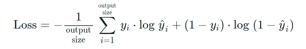
说明:
- yi: 是真实值
- y_hat: 预测值
- output size: 图片的个数,如:图片shape: (batch,height,width,channel) , 那就是他们4个数的乘积。
1.2 数据验证
import os

os.environ['TF_CPP_MIN_LOG_LEVEL'] = '2'
import tensorflow as tf
from tensorflow.keras.losses import BinaryCrossentropy
import numpy as np

loss = BinaryCrossentropy()
1.2.1 一维
# 一维
y_true = np.array([0, 1, 1])
y_pred = np.array([0.6, 0.4, 0.3])
- tf
loss_result_1 = loss(y_true, y_pred)
print('交叉熵计算:', loss_result_1)

2. numpy
np_result_1 = y_true * np.log(y_pred) + (1 - y_true) * np.log(1 - y_pred)
np_result_1 = -np.sum(np_result_1)/y_true.size
print('numpy计算:', np_result_1)
- 单个元素计算
每个对应的值进行计算
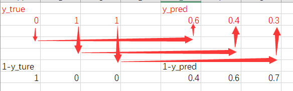
# 3. 单个元素计算
temp = -(1*np.log(0.4)+1*np.log(0.4)+1*np.log(0.3))/3
print('单个元素计算:', temp)

1.2.2 二维
y_true = np.array([[0, 1], [0, 0]])
y_pred = np.array([[0.2, 0.9], [0.1, 0.2]])
- tf
loss_result_1 = loss(y_true, y_pred)
print('交叉熵计算:', loss_result_1)

- numpy
np_result_1 = y_true * np.log(y_pred) + (1 - y_true) * np.log(1 - y_pred)
np_result_1 = -np.sum(np_result_1) / y_true.size
print('numpy计算:', np_result_1)

3. 单个元素计算
temp = -(1 * np.log(0.8) + 1 * np.log(0.9) + 1 * np.log(0.9)+ 1 * np.log(0.8)) / 4
print('单个元素计算:', temp)

1.2.3 小结
以图片分割为例:
图片shape: (batch,height,width,channel)
- 上篇文章中Crossentropy是对通道方向上进行计算,损失=总和/(batch+height+width)。
- 本文的BinaryCrossentropy对每个值进行计算,损失=总和/(batch+height+width+channel)