关于这部分的理论知识可以参考我的这篇博客《特征值与特征向量》定义、意义及例子,下面主要介绍如何计算方阵的特征值和特征向量

1.np.linalg.eig()

计算方阵的特征值和特征向量，numpy提供了接口eig，直接调用就行，下面主要介绍该函数：

该函数的原型如下：

def eig(a):
	Parameters
	----------
	a : (..., M, M) array
	Matrices for which the eigenvalues and right eigenvectors will
	be computed

	Returns
    -------
    w : (..., M) array
        The eigenvalues, each repeated according to its multiplicity.
        The eigenvalues are not necessarily ordered. The resulting
        array will be of complex type, unless the imaginary part is
        zero in which case it will be cast to a real type. When `a`
        is real the resulting eigenvalues will be real (0 imaginary
        part) or occur in conjugate pairs

    v : (..., M, M) array
        The normalized (unit "length") eigenvectors, such that the
        column ``v[:,i]`` is the eigenvector corresponding to the
        eigenvalue ``w[i]``.

可以看出，该函数的参数只有一个，也就是我们要求特征值和特征向量的方阵（只有方阵才有特征值和特征向量），该函数的返回值有两个分别为w和v。

w: 代表特征值
返回值w是一个一维的array，w的长度和方阵的维度是相同的，对于一个m x m的方阵，其特征值的个数也为m，另外注意不一定特征值不一定是有序排列。

v: 代表特征向量
返回值v是一个array类型的数据，其维度和方阵的维度是相同的，对于一个m x m的方阵，v的维度也为m x m，v中包含m个特征向量，每个特征向量的长度为m，v[:,i]对应特征值为w[i]的特征向量，特征向量是进行单位化（除以所有元素的平方和的开方）的形式。

2.例子

下面举例说明一下：

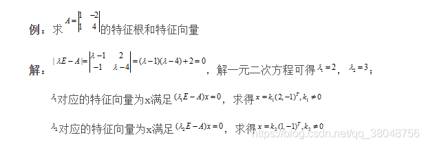
对于上面的这样一个例子，直接转化为代码：

>>> import numpy as np
>>> a = np.array([[1, -2], [1, 4]])
>>> a
array([[ 1, -2],
       [ 1,  4]])
>>> np.linalg.eig(a)
(array([2., 3.]), array([[-0.89442719,  0.70710678],
       [ 0.4472136 , -0.70710678]]))
>>>

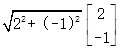
可以看出求得的特征值为[2, 3],特征向量为[-0.89442719, 0.4472136] 与[0.70710678, -0.70710678]，很明显特征向量进行了单位化，例如第一个特征向量的单位化如下：

3. 应用

对于求特征值与特征向量的应用，最常见的就是对称矩阵的对角化，对于实对称矩阵A，可以对角化转化为下式

转换后的式中p以及对角阵的求取，就可以利用np.linalg.eig()

diag, p = np.linalg.eig(A)

关于对称矩阵对角化的具体求法可以参考这篇博客对称矩阵的对角化.

4.其他例子

官方还给出了一起其他的例子，包括特征值是复数的例子如下：

from numpy import linalg as LA
(Almost) trivial example with real e-values and e-vectors.

>>>
w, v = LA.eig(np.diag((1, 2, 3)))
w; v
array([1., 2., 3.])
array([[1., 0., 0.],
       [0., 1., 0.],
       [0., 0., 1.]])
Real matrix possessing complex e-values and e-vectors; note that the e-values are complex conjugates of each other.

>>>
w, v = LA.eig(np.array([[1, -1], [1, 1]]))
w; v
array([1.+1.j, 1.-1.j])
array([[0.70710678+0.j        , 0.70710678-0.j        ],
       [0.        -0.70710678j, 0.        +0.70710678j]])
Complex-valued matrix with real e-values (but complex-valued e-vectors); note that a.conj().T == a, i.e., a is Hermitian.

>>>
a = np.array([[1, 1j], [-1j, 1]])
w, v = LA.eig(a)
w; v
array([2.+0.j, 0.+0.j])
array([[ 0.        +0.70710678j,  0.70710678+0.j        ], # may vary
       [ 0.70710678+0.j        , -0.        +0.70710678j]])
Be careful about round-off error!

>>>
a = np.array([[1 + 1e-9, 0], [0, 1 - 1e-9]])
# Theor. e-values are 1 +/- 1e-9
w, v = LA.eig(a)
w; v
array([1., 1.])
array([[1., 0.],
       [0., 1.]])

5.官方完整说明

官方的apihttps://numpy.org/doc/stable/reference/generated/numpy.linalg.eig.html

完整的说明我也给放在了下面

    """
    Compute the eigenvalues and right eigenvectors of a square array.

    Parameters
    ----------
    a : (..., M, M) array
        Matrices for which the eigenvalues and right eigenvectors will
        be computed

    Returns
    -------
    w : (..., M) array
        The eigenvalues, each repeated according to its multiplicity.
        The eigenvalues are not necessarily ordered. The resulting
        array will be of complex type, unless the imaginary part is
        zero in which case it will be cast to a real type. When `a`
        is real the resulting eigenvalues will be real (0 imaginary
        part) or occur in conjugate pairs

    v : (..., M, M) array
        The normalized (unit "length") eigenvectors, such that the
        column ``v[:,i]`` is the eigenvector corresponding to the
        eigenvalue ``w[i]``.

    Raises
    ------
    LinAlgError
        If the eigenvalue computation does not converge.

    See Also
    --------
    eigvals : eigenvalues of a non-symmetric array.
    eigh : eigenvalues and eigenvectors of a real symmetric or complex
           Hermitian (conjugate symmetric) array.
    eigvalsh : eigenvalues of a real symmetric or complex Hermitian
               (conjugate symmetric) array.
    scipy.linalg.eig : Similar function in SciPy that also solves the
                       generalized eigenvalue problem.
    scipy.linalg.schur : Best choice for unitary and other non-Hermitian
                         normal matrices.

    Notes
    -----

    .. versionadded:: 1.8.0

    Broadcasting rules apply, see the `numpy.linalg` documentation for
    details.

    This is implemented using the ``_geev`` LAPACK routines which compute
    the eigenvalues and eigenvectors of general square arrays.

    The number `w` is an eigenvalue of `a` if there exists a vector
    `v` such that ``a @ v = w * v``. Thus, the arrays `a`, `w`, and
    `v` satisfy the equations ``a @ v[:,i] = w[i] * v[:,i]``
    for :math:`i \\in \\{0,...,M-1\\}`.

    The array `v` of eigenvectors may not be of maximum rank, that is, some
    of the columns may be linearly dependent, although round-off error may
    obscure that fact. If the eigenvalues are all different, then theoretically
    the eigenvectors are linearly independent and `a` can be diagonalized by
    a similarity transformation using `v`, i.e, ``inv(v) @ a @ v`` is diagonal.

    For non-Hermitian normal matrices the SciPy function `scipy.linalg.schur`
    is preferred because the matrix `v` is guaranteed to be unitary, which is
    not the case when using `eig`. The Schur factorization produces an
    upper triangular matrix rather than a diagonal matrix, but for normal
    matrices only the diagonal of the upper triangular matrix is needed, the
    rest is roundoff error.

    Finally, it is emphasized that `v` consists of the *right* (as in
    right-hand side) eigenvectors of `a`.  A vector `y` satisfying
    ``y.T @ a = z * y.T`` for some number `z` is called a *left*
    eigenvector of `a`, and, in general, the left and right eigenvectors
    of a matrix are not necessarily the (perhaps conjugate) transposes
    of each other.

    References
    ----------
    G. Strang, *Linear Algebra and Its Applications*, 2nd Ed., Orlando, FL,
    Academic Press, Inc., 1980, Various pp.

    Examples
    --------
    >>> from numpy import linalg as LA

    (Almost) trivial example with real e-values and e-vectors.

    >>> w, v = LA.eig(np.diag((1, 2, 3)))
    >>> w; v
    array([1., 2., 3.])
    array([[1., 0., 0.],
           [0., 1., 0.],
           [0., 0., 1.]])

    Real matrix possessing complex e-values and e-vectors; note that the
    e-values are complex conjugates of each other.

    >>> w, v = LA.eig(np.array([[1, -1], [1, 1]]))
    >>> w; v
    array([1.+1.j, 1.-1.j])
    array([[0.70710678+0.j        , 0.70710678-0.j        ],
           [0.        -0.70710678j, 0.        +0.70710678j]])

    Complex-valued matrix with real e-values (but complex-valued e-vectors);
    note that ``a.conj().T == a``, i.e., `a` is Hermitian.

    >>> a = np.array([[1, 1j], [-1j, 1]])
    >>> w, v = LA.eig(a)
    >>> w; v
    array([2.+0.j, 0.+0.j])
    array([[ 0.        +0.70710678j,  0.70710678+0.j        ], # may vary
           [ 0.70710678+0.j        , -0.        +0.70710678j]])

    Be careful about round-off error!

    >>> a = np.array([[1 + 1e-9, 0], [0, 1 - 1e-9]])
    >>> # Theor. e-values are 1 +/- 1e-9
    >>> w, v = LA.eig(a)
    >>> w; v
    array([1., 1.])
    array([[1., 0.],
           [0., 1.]])

    """