1)均方误差(mean squared error)
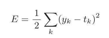

程序实现
def mean_squared_error(y, t):
    return 0.5 * np.sum((y-t)**2)
举例:
    t = [0, 0, 1, 0, 0, 0, 0, 0, 0, 0]#假设第二个位置为正确值,ont-hot显示
    y1 = [0.1, 0.05, 0.6, 0.0, 0.05, 0.1, 0.0, 0.1, 0.0, 0.0]#实际的向量,2的概率最大
    val = mean_squared_error(np.array(y1), np.array(t))
    print(val)#0.09750000000000003  均方差比较小

    y2 = [0.1, 0.05, 0.1, 0.0, 0.05, 0.1, 0.0, 0.6, 0.0, 0.0]#7的位置 概率最大
    val = mean_squared_error(np.array(y2), np.array(t))
    print(val)#0.5975  均方差比较大
    #由此可见y1 与目标值相近
2)交叉熵误差
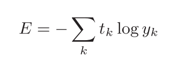
yk是神经网络的输出, tk是正确解标签。
交叉熵误差的值是由正确解标签所对应的输出结果决定的。
正确解标签对应的输出越大,值越接近0;当输出为1时,交叉熵误差为0。此外,如果正确解标签对应的输出较小,则式子的值较大。
def cross_entropy_error(y, t):
	delta = 1e-7
	return -np.sum(t * np.log(y + delta))
举例说明
    t = [0, 0, 1, 0, 0, 0, 0, 0, 0, 0]  # 假设第二个位置为正确值,ont-hot显示
    y1 = [0.1, 0.05, 0.6, 0.0, 0.05, 0.1, 0.0, 0.1, 0.0, 0.0]  # 实际的向量,2的概率最大
    val = cross_entropy_error(np.array(y1), np.array(t))
    print(val)#0.510825457099338

    y2 = [0.1, 0.05, 0.1, 0.0, 0.05, 0.1, 0.0, 0.6, 0.0, 0.0]#7的位置 概率最大
    val = cross_entropy_error(np.array(y2), np.array(t))
    print(val)#2.302584092994546
2)批量处理
one-hot形式
def cross_entroy_error(y,t):
    if y.ndim == 1:
        t = t.reshape(1,t.size)#转化为二维
        y = y.reshape(1,y.size)
    batch_size = y.shape[0]
    return -np.sum(t*np.log(y+1e-7))/batch_size
非one-hot形式
def cross_entroy_error(y,t):
    if y.ndim == 1:
        t = t.reshape(1,t.size)
        y = y.reshape(1,y.size)
    batch_size = y.shape[0]
    return -np.sum(np.log(y[np.arrange(batch_size),t]+1e-7))/batch_size
    #np.log(y[np.arrange(batch_size),t]+1e-7)
如果可以获得神经网络在正确解标签处的输出,就可以计算交叉熵误差。因此, t为 one-hot表示时通过t * np.log(y)计算的地方,在 t为标签形式时,可用 np.log( y[np.arange(batch_size), t] )实现相同的处理。