一次读取FY4A雷电数据（LMI）的过程总结

本帖介绍了一次作者读取FY4A雷电数据（LMI）的过程，介绍了一步一步怎么把自己从来没有碰到过的数据读取出来，涉及了一个库netCDF4，对于会的朋友没有任何知识点和借鉴意义，可以不看的，只在给新手小白朋友们去讲解当拿到一种数据之后该怎么一步一步把它读出来

一、数据来源

来自于以为网友，让我尝试读一下，文件名：FY4A-_LMI—_N_REGX_1047E_L2-_LMIE_SING_NUL_20200701000000_20200701000449_7800M_N01V1.NC
事先告诉了我这是雷电数据。

二、第一步尝试

第一眼看到是NC后缀的文件，所以想利用《小白学习cartopy气象画地图的第二天》读取温度的方式进行读取，即：

import xarray as xr
ds = xr.open_dataset('FY4A-_LMI---_N_REGX_1047E_L2-_LMIE_SING_NUL_20200701000000_20200701000449_7800M_N02V1.NC')

运行结果：
SerializationWarning: variable ‘EYP’ has _Unsigned attribute but is not of integer type. Ignoring attribute.
new_vars[k] = decode_cf_variable(
进程已结束,退出代码0

从结果来看，程序跑结束了，返回值0，虽然报了很多警告，但是没有报错，说明数据可能读出来了。

三、第二步打印

print(ds)

运行结果：
<xarray.Dataset>
Dimensions: (o: 1, x: 36)
Dimensions without coordinates: o, x
Data variables:
LON (x) float32 …
LAT (x) float32 …
EOT (x) float32 …
ER (x) float32 …
EFP (x) float32 …
EA (x) float32 …
EGA (x) float32 …
EXP (x) float32 …
EYP (x) float32 …
DQF (x) int8 …
nominal_satellite_subpoint_lat (o) float32 …
nominal_satellite_subpoint_lon (o) float32 …
nominal_satellite_height (o) float32 …
geospatial_lat_lon_extent (o) float32 …
OBIType (o) int32 …
processing_parm_version_container (o) int32 …
algorithm_product_version_container (o) int32 …
。。。。。。。。。。。。。

一大串英文加数字，咱们不一定能看懂，但是有两个东西值得注意LON、LAT，经纬度嘛。那这里面是不是就是存着数据呢，对应上下文，是不是一个以（x）为下标的数组，一组经度，一组纬度，然后下面就是各种物理量，上文提示了总共36个。然后再下面是以（o）为下标的，就一个。那么Data variables就是数据的意思。

四、第三步打印数据

print(ds.variables)

运行结果：
Frozen({‘LON’: <xarray.Variable (x: 36)>
array([82.64, 82.62, 82.57, 82.46, 82.48, 82.66, 82.64, 82.62, 82.57, 82.46,
82.48, 82.66, 82.53, 82.71, 82.51, 82.73, 82.6 , 82.59, 82.42, 82.64,
82.57, 82.46, 82.48, 82.66, 82.62, 82.53, 82.73, 98.07, 98.15, 98.07,
98.15, 98.14, 98.07, 97.99, 98.07, 98.15], dtype=float32)
。。。
‘LAT’: <xarray.Variable (x: 36)>
array([25.73, 25.82, 25.65, 25.73, 25.65, 25.65, 25.73, 25.82, 25.65, 25.73,
25.65, 25.65, 25.82, 25.81, 25.9 , 25.73, 25.9 , 25.56, 25.9 , 25.73,
25.65, 25.73, 25.65, 25.65, 25.82, 25.82, 25.73, 21.54, 21.47, 21.54,
21.47, 21.55, 21.46, 21.54, 21.54, 21.47], dtype=float32)
。。。})

仔细看，这其实是不是就是一个python的字典，那么就直接引出咱们的第四步了

五、第四步打印字典

print(ds.variables['LON'])

运行结果：
<xarray.Variable (x: 36)>
array([82.64, 82.62, 82.57, 82.46, 82.48, 82.66, 82.64, 82.62, 82.57, 82.46,
82.48, 82.66, 82.53, 82.71, 82.51, 82.73, 82.6 , 82.59, 82.42, 82.64,
82.57, 82.46, 82.48, 82.66, 82.62, 82.53, 82.73, 98.07, 98.15, 98.07,
98.15, 98.14, 98.07, 97.99, 98.07, 98.15], dtype=float32)
Attributes:
long_name: Event Longitude
standard_name: Event Longitude
FillValue: 65535.0
valid_range: [-180. 180.]
units: degree
resolution: 7800m
coordinates: x
ancillary_variables: DQF
Description: China

从结果来看，确实有一个数组，存的应该是经度信息，下面还有另外一些类似解释说明的信息（Attributes属性），这时候可能就在担心这些信息是否会影响我们读取数据。先不管啦，既然是数组，那么是否可以按下标索引呢？

六、第五步打印单个数据

print(ds.variables['LON'][0])

运行结果：
<xarray.Variable ()>
array(82.64, dtype=float32)
Attributes:
long_name: Event Longitude
standard_name: Event Longitude
FillValue: 65535.0
valid_range: [-180. 180.]
units: degree
resolution: 7800m
coordinates: x
ancillary_variables: DQF
Description: China

出现了第四步里面的第0个元素，虽然仍然跟着属性，咱们暂时先不管他，意味着ds.variables[‘LON’]里面就是经度信息。那么其他的各个数据存放应该也是类似的规律。
拿着经纬度，利用散点图，是否就可以画出闪电的位置了呢？下面开始尝试。这里解释一下，上面的很多步骤都是用来摸清文件里面的数据结构，提取我们需要的数据。

七、第六步提取数据

根据上面的经验，我们可以写这样的代码

import xarray as xr
ds = xr.open_dataset('FY4A-_LMI---_N_REGX_1047E_L2-_LMIE_SING_NUL_20200701000000_20200701000449_7800M_N02V1.NC')
lon = ds.variables['LON']
lat = ds.variables['LAT']

这样我们就得到了闪电事件的位置，弄一张地图，再画个散点图，理论上应该就成功了。

八、第七步画图

画地图部分参照《小白学习cartopy气象画地图的第二天》这里就不做具体解释了，画好地图后利用

ax.scatter(lon, lat, s=350, alpha=.6)

画图

发现并没有数据，可能性很多，就像最初怀疑数据有问题，那么，咱们不使用数据，直接输入一个经纬度（105,35）看看是否有结果

ax.scatter(105, 35, s=350, alpha=.6)

发现依旧没有结果，说明不是数据的问题，尝试加入投影参数

ax.scatter(lon, lat, s=350, alpha=.6,transform=ccrs.PlateCarree())

数据出现了，按最初的规律，应该是32个点，这里并没有。仔细看图，发现这两个点并不是圆，放大发现：

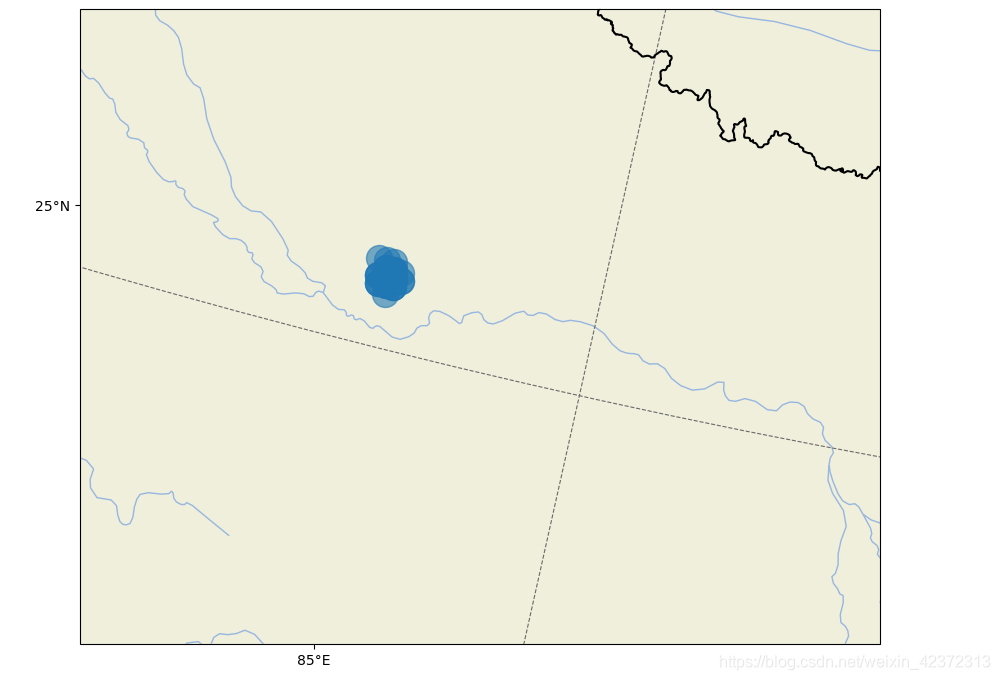
是有很多个点叠加的结果，应该是点的大小设置过大造成的。修改代码

ax.scatter(lon, lat, s=5, alpha=.6,transform=ccrs.PlateCarree())

至此，闪电位置标记成功。就此结束了吗，并没有，在最初找数据的过程中，我们发现了还有很多其他的量，比如EOT、ER、EFP、EA、EGA 这些都代表了什么呢？两条路，一条就是直接百度，第二条，就是去搞懂数据结构。

九、第八步查找数据结构

其实，拿到一个数据，最先搞明白的就是这个数据的结构，每个字节代表了什么意思。python好就好在很多通用的格式已经帮我们写好了读取方法，就比如这次帖子里面的数据。但是我们也要做好最坏的打算，万一没有普适性的方法，需要我们自己按字节去读取。
这里提供一个案例：《小白学习Basemap气象画地图的第五天（读取micaps站点数据，省级能见度分布）》，里面的read_mdfs.py就是按照micaps的格式文档，按字节读取的micaps数据，推荐对照文档研究一下。
拿到FY4A雷电数据之后，通过这种论坛，七拐八拐来到了

网址：http://data.nsmc.org.cn/portalsite/default.aspx
在里面找到了

闪电仪的数据格式（可下载），这个网址还能下载风云数据

这里就有各个物理量的解释。当然，还是需要自己去翻译。
至此，单个数据文件我是怎么读出来的过程也介绍完毕了。

十、一些补充

1.因为网友给的不只是一个文件，所以下面给大家的py文件里面还有一些文件读取和循环的操作，我会注释好。
出图：


2.由于网友的要求，测试数据就不给大家了，但是上文提到的网站都能下载到，大家可以自行去下载。
3.这里做的是全国及其周边的，没有特地去做一个省的图，其实也很简单，两种方法，一种是画好全国，然后做掩膜，还有一种是在数据读取阶段做一个筛选，利用经纬度把不在范围内的数据剔除。
4.本帖的目前是教会大家怎么去读取一个数据，怎么下手，所以写的段落符合思维顺序，不符合阅读顺序。
5.出的图没有做修饰，也没有很美观，因为目的不在于此，大家可以自己美化，比如闪电位置用“+”，写上时间等等。授人以鱼不如授人以渔。
6.我因为最开始以为xarray读取失败，所以最先研究的是数据格式文档，发现了数据格式为NetCDF,因此使用的库是netCDF4，前者更底层，后者更专业，结果都一样。

7.要画风云4云图靠这些还不够，还有很多东西要去搞懂，但思路是差不多的，别头大就好。
8.最坏的情况就是逐字节去读取，但是前提也是需要先知道数据格式。要学会看数据格式

完整代码

from netCDF4 import Dataset
import os
import matplotlib.pyplot as plt
import numpy as np
from copy import copy
import cartopy.crs as ccrs
import cartopy.feature as cfeature
from cartopy.mpl.gridliner import LATITUDE_FORMATTER, LONGITUDE_FORMATTER
import shapely.geometry as sgeom



#给画刻度用来辅助，确定四周
def find_side(ls, side):
    """
 Given a shapely LineString which is assumed to be rectangular, return the
 line corresponding to a given side of the rectangle.

 """
    minx, miny, maxx, maxy = ls.bounds
    points = {
    
    'left': [(minx, miny), (minx, maxy)],
              'right': [(maxx, miny), (maxx, maxy)],
              'bottom': [(minx, miny), (maxx, miny)],
              'top': [(minx, maxy), (maxx, maxy)],}
    return sgeom.LineString(points[side])
#用来画坐标轴的刻度（包括经度和纬度）
def _lambert_ticks(ax, ticks, tick_location, line_constructor, tick_extractor):
    """得到一个兰伯特正形投影的轴的刻度位置和标签."""
    outline_patch = sgeom.LineString(ax.outline_patch.get_path().vertices.tolist())
    axis = find_side(outline_patch, tick_location)
    n_steps = 30
    extent = ax.get_extent(ccrs.PlateCarree())
    _ticks = []
    for t in ticks:
        xy = line_constructor(t, n_steps, extent)
        proj_xyz = ax.projection.transform_points(ccrs.Geodetic(), xy[:, 0], xy[:, 1])
        xyt = proj_xyz[..., :2]
        ls = sgeom.LineString(xyt.tolist())
        locs = axis.intersection(ls)
        if not locs:
            tick = [None]
        else:
            tick = tick_extractor(locs.xy)
        _ticks.append(tick[0])
    # Remove ticks that aren't visible:
    ticklabels = copy(ticks)
    while True:
        try:
            index = _ticks.index(None)
        except ValueError:
            break
        _ticks.pop(index)
        ticklabels.pop(index)
    return _ticks, ticklabels
#设置x轴标签（用来画纬度）
def lambert_xticks(ax, ticks):
    """Draw ticks on the bottom x-axis of a Lambert Conformal projection."""
    te = lambda xy: xy[0]
    lc = lambda t, n, b: np.vstack((np.zeros(n) + t, np.linspace(b[2], b[3], n))).T
    xticks, xticklabels = _lambert_ticks(ax, ticks, 'bottom', lc, te)
    ax.xaxis.tick_bottom()
    ax.set_xticks(xticks)
    ax.set_xticklabels([ax.xaxis.get_major_formatter()(xtick) for xtick in xticklabels])
#设置y轴标签（用来画经度）
def lambert_yticks(ax, ticks):
    """Draw ricks on the left y-axis of a Lamber Conformal projection."""
    te = lambda xy: xy[1]
    lc = lambda t, n, b: np.vstack((np.linspace(b[0], b[1], n), np.zeros(n) + t)).T
    yticks, yticklabels = _lambert_ticks(ax, ticks, 'left', lc, te)
    ax.yaxis.tick_left()
    ax.set_yticks(yticks)
    ax.set_yticklabels([ax.yaxis.get_major_formatter()(ytick) for ytick in yticklabels])
#获得所有文件的绝对路径
def get_files_path_list(path):
    files = []
    filesList = os.listdir(path)
    for filename in filesList:
        fileAbsPath = os.path.join(path,filename)
        files.append(fileAbsPath)
    return files
#画闪电位置
def drow(ax,files_path):
    #从列表中取出每一个文件路径，画图
    for file in files_path:
        nc_file = Dataset(file, 'r')
        lon = list(nc_file.variables['LON'][:])
        lat = list(nc_file.variables['LAT'][:])
        # er = list(nc_file.variables['ER'][:])#光辉
        ax.scatter(lon, lat, s=5, alpha=.6,transform=ccrs.PlateCarree())



#-------------------画地图部分----------#
fig = plt.figure(figsize=[10, 8],frameon=True)
#给画图区添加兰伯特投影
ax = fig.add_axes([0.08, 0.05, 0.8, 0.94], projection=ccrs.LambertConformal(central_latitude=90, central_longitude=105))

ax.add_feature(cfeature.OCEAN.with_scale('50m'))
ax.add_feature(cfeature.LAND.with_scale('50m'))
ax.add_feature(cfeature.RIVERS.with_scale('50m'))
ax.add_feature(cfeature.LAKES.with_scale('50m'))

ax.set_extent([80, 130, 15, 55],crs=ccrs.PlateCarree())
fig.canvas.draw()

#设置刻度值，画经纬网格
xticks = [55, 65, 75, 85, 95, 105, 115, 125, 135, 145, 155, 165]
yticks = [0 , 5 , 10, 15, 20, 25 , 30 , 35 , 40 , 45 , 50 , 55 , 60 , 65]
ax.gridlines(xlocs=xticks, ylocs=yticks,linestyle='--',lw=1,color='dimgrey')

# 设置经纬网格的端点（也是用来配合画刻度的，注释掉以后刻度不能正常显示了）
ax.xaxis.set_major_formatter(LONGITUDE_FORMATTER)
ax.yaxis.set_major_formatter(LATITUDE_FORMATTER)
#画经纬度刻度
lambert_xticks(ax, xticks)
lambert_yticks(ax, yticks)


with open('CN-border-La.dat') as src:
    context = src.read()
    blocks = [cnt for cnt in context.split('>') if len(cnt) > 0]
    borders = [np.fromstring(block, dtype=float, sep=' ') for block in blocks]
for line in borders:
    ax.plot(line[0::2], line[1::2], '-', lw=1.5, color='k',
            transform=ccrs.Geodetic())
#-------------------画地图部分----------#


#------------读取数据画图部分-------------#
#数据文件夹位置
path = r'D:\project\study_way\cartopy\A2021011103078357900001\A2021011103078357900001'
#获取文件的绝对路径列表
files_path = get_files_path_list(path)
#画图
drow(ax,files_path)
#------------读取数据画图部分-------------#




#出图
plt.show()