学习来源：日撸 Java 三百行（51-60天，kNN 与 NB）_闵帆的博客-CSDN博客

符号型数据的 NB 算法

符号型数据是指数据集中的数据是由字符或者字符串构成. NB (Native Bayes) 算法通常被翻译成朴素贝叶斯算法, 基于贝叶斯算法, 常用于分类问题. 同时这也是贝叶斯算法中最简单、最常见的一种.

一、 符号型数据集

在 https://gitee.com/fansmale/javasampledata 中可以获得 weather.arff 文件.

@relation weather
@attribute Outlook {Sunny, Overcast, Rain}
@attribute Temperature {Hot, Mild, Cool}
@attribute Humidity {High, Normal, Low}
@attribute Windy {FALSE, TRUE}
@attribute Play {N, P}
@data
Sunny,Hot,High,FALSE,N
Sunny,Hot,High,TRUE,N
Overcast,Hot,High,FALSE,P
Rain,Mild,High,FALSE,P
Rain,Cool,Normal,FALSE,P
Rain,Cool,Normal,TRUE,N
Overcast,Cool,Normal,TRUE,P
Sunny,Mild,High,FALSE,N
Sunny,Cool,Normal,FALSE,P
Rain,Mild,Normal,FALSE,P
Sunny,Mild,Normal,TRUE,P
Overcast,Mild,High,TRUE,P
Overcast,Hot,Normal,FALSE,P
Rain,Mild,High,TRUE,N

文件中对 weather 有 Outlook、Temperature、Humidity、Windy 和 Play 五个属性. 在五个属性中存在着具体的描述, 我们的任务就是要通过除 Play 之外的所有属性来预测 Play 的值. 也就是说这还是一个分类问题, 但是获得的数据就不再是之前的数值, 而是一段描述字符串.

二、 理论推导

1. 条件概率

$$P(AB)=P(A)P(B|A)\text{\hspace{1em}(1)}$$

• $P(A)$ 表示事件 $A$ 发生的概率.
• $P(AB)$ 表示事件 $A$ 和 事件$B$ 同时发生的概率.
• $P(B|A)$ 表示在事件 $A$ 发生的情况下, 事件$B$也发生的概率.

例: $A$ 表示天气是晴天, 即 Outlook = Sunny; $B$ 表示湿度高, 即 Humidity = High.

14 天中有 5 天为 Sunny , 则 $P(A)=P(Outlook=Sunny)=5/14$

在 5 天为 Sunny 中又有 3 天湿度高, 则有 $P(B|A)=P(Humidity=High|Outlook=Sunny)=3/5$

最后我们就能得到即是晴天又湿度高的概率 $P(AB)=P(Outlook=Sunny\wedge Humidity=High)=P(A)P(B|A)=3/14$

2. 独立性假设

令 $\mathrm{x} = x_1 \wedge x_2 \wedge … \wedge x_m $ 表示一个条件的组合, 如 Play = Sunny $\wedge$ Hot $\wedge$ High $\wedge$ FALSE = N.

令 $D$ 表示一个事件, 如：Play = N, 根据 (1) 式有:

$$P(D|\mathrm{x})=\frac{P(\mathrm{x}D)}{P(\mathrm{x})}=\frac{P(D)P(\mathrm{x}|D)}{P(\mathrm{x})}\text{\hspace{1em}(2)}$$

接下来就是一个非常精彩的操作, 我们假设 $x_1,x_2,...,x_m$ 它们之间相互独立. 这在现实世界中就显得有些荒谬. 比如阴天容易刮风, 晴天湿度低. 这里姑且算其成立.

$$P(\mathrm{x}|D)=P(x_1|D)P(x_2|D)...P(x_m|D)=\prod _{i=1}^{m}P(x_i|D)\text{\hspace{1em}(3)}$$

综合 (2) (3) 式可得:

$$P(D|\mathrm{x})=\frac{P(\mathrm{x}D)}{P(\mathrm{x})}=\frac{P(D){\prod }_{i=1}^{m}P(x_i|D)}{P(\mathrm{x})}\text{\hspace{1em}(4)}$$

因为计算不了分母 $P(\mathrm{x})$ 所以我们就只需要比较分子大小, 谁大归哪个类.

3. Laplacian 平滑

由于数据集中不能保证每个数据都出现, 若是按照以上算法就会导致出现 0 的情况. 但是在现实世界中真实存在着导致结果为 0 的数据, 我们自然不希望这样的事情发生. 所以 Laplacian 平滑由此诞生.

$$P^L(x_i|D)=\frac{nP(x_{i}D)+1}{nP(D)+v_i}\text{\hspace{1em}(5)}$$

其中 n 表示数据集中所有数据的个数, $v_i$ 表示第 $i$ 个属性的可能取值数. 如 i 表示 Humidity 属性时, $v_i=3$.

三、 代码流程

1. 具体代码

package bayes;

import java.io.FileReader;
import java.util.Arrays;

import weka.core.*;

/**
 * The Naive Bayes algorithm.
 *
 * @author Shi-Huai Wen Email: [email protected].
 */


public class NaiveBayes {
    
    

    /**
     * The data.
     */
    Instances dataset;

    /**
     * The number of classes. For binary classification it is 2.
     */
    int numClasses;

    /**
     * The number of instances.
     */
    int numInstances;

    /**
     * The number of conditional attributes.
     */
    int numConditions;

    /**
     * The prediction, including queried and predicted labels.
     */
    int[] predicts;

    /**
     * Class distribution.
     */
    double[] classDistribution;

    /**
     * Class distribution with Laplacian smooth.
     */
    double[] classDistributionLaplacian;

    /**
     * To calculate the conditional probabilities for all classes over all
     * attributes on all values.
     */
    double[][][] conditionalCounts;

    /**
     * The conditional probabilities with Laplacian smooth.
     */
    double[][][] conditionalProbabilitiesLaplacian;

    /**
     * Data type.
     */
    int dataType;

    /**
     * Nominal.
     */
    public static final int NOMINAL = 0;

    /**
     * *******************
     * The constructor.
     *
     * @param paraFilename The given file.
     * *******************
     */
    public NaiveBayes(String paraFilename) {
    
    
        dataset = null;
        try {
    
    
            FileReader fileReader = new FileReader(paraFilename);
            dataset = new Instances(fileReader);
            fileReader.close();
        } catch (Exception ee) {
    
    
            System.out.println("Cannot read the file: " + paraFilename + "\r\n" + ee);
            System.exit(0);
        } // Of try

        dataset.setClassIndex(dataset.numAttributes() - 1);
        numConditions = dataset.numAttributes() - 1;
        numInstances = dataset.numInstances();
        numClasses = dataset.attribute(numConditions).numValues();
    }// Of the constructor

    /**
     * *******************
     * Set the data type.
     * *******************
     */
    public void setDataType(int paraDataType) {
    
    
        dataType = paraDataType;
    }// Of setDataType

    /**
     * *******************
     * Calculate the class distribution with Laplacian smooth.
     * *******************
     */
    public void calculateClassDistribution() {
    
    
        classDistribution = new double[numClasses];
        classDistributionLaplacian = new double[numClasses];

        double[] tempCounts = new double[numClasses];
        for (int i = 0; i < numInstances; i++) {
    
    
            int tempClassValue = (int) dataset.instance(i).classValue();
            tempCounts[tempClassValue]++;
        } // Of for i

        for (int i = 0; i < numClasses; i++) {
    
    
            classDistribution[i] = tempCounts[i] / numInstances;
            classDistributionLaplacian[i] = (tempCounts[i] + 1) / (numInstances + numClasses);
        } // Of for i

        System.out.println("Class distribution: " + Arrays.toString(classDistribution));
        System.out.println(
                "Class distribution Laplacian: " + Arrays.toString(classDistributionLaplacian));
    }// Of calculateClassDistribution

    /**
     * *******************
     * Calculate the conditional probabilities with Laplacian smooth. ONLY scan
     * the dataset once. There was a simpler one, I have removed it because the
     * time complexity is higher.
     * *******************
     */
    public void calculateConditionalProbabilities() {
    
    
        conditionalCounts = new double[numClasses][numConditions][];
        conditionalProbabilitiesLaplacian = new double[numClasses][numConditions][];

        // Allocate space
        for (int i = 0; i < numClasses; i++) {
    
    
            for (int j = 0; j < numConditions; j++) {
    
    
                int tempNumValues = dataset.attribute(j).numValues();
                conditionalCounts[i][j] = new double[tempNumValues];
                conditionalProbabilitiesLaplacian[i][j] = new double[tempNumValues];
            } // Of for j
        } // Of for i

        // Count the numbers
        int[] tempClassCounts = new int[numClasses];
        for (int i = 0; i < numInstances; i++) {
    
    
            int tempClass = (int) dataset.instance(i).classValue();
            tempClassCounts[tempClass]++;
            for (int j = 0; j < numConditions; j++) {
    
    
                int tempValue = (int) dataset.instance(i).value(j);
                conditionalCounts[tempClass][j][tempValue]++;
            } // Of for j
        } // Of for i

        // Now for the real probability with Laplacian
        for (int i = 0; i < numClasses; i++) {
    
    
            for (int j = 0; j < numConditions; j++) {
    
    
                int tempNumValues = dataset.attribute(j).numValues();
                for (int k = 0; k < tempNumValues; k++) {
    
    
                    conditionalProbabilitiesLaplacian[i][j][k] = (conditionalCounts[i][j][k] + 1)
                            / (tempClassCounts[i] + tempNumValues);
                } // Of for k
            } // Of for j
        } // Of for i

        System.out.println("Conditional probabilities: " + Arrays.deepToString(conditionalCounts));
    }// Of calculateConditionalProbabilities

    /**
     * *******************
     * Classify all instances, the results are stored in predicts[].
     * *******************
     */
    public void classify() {
    
    
        predicts = new int[numInstances];
        for (int i = 0; i < numInstances; i++) {
    
    
            predicts[i] = classify(dataset.instance(i));
        } // Of for i
    }// Of classify

    /**
     * *******************
     * Classify an instances.
     * *******************
     */
    public int classify(Instance paraInstance) {
    
    
        if (dataType == NOMINAL) {
    
    
            return classifyNominal(paraInstance);
        }
        return -1;
    }// Of classify

    /**
     * *******************
     * Classify an instances with nominal data.
     * *******************
     */
    public int classifyNominal(Instance paraInstance) {
    
    
        // Find the biggest one
        double tempBiggest = -10000;
        int resultBestIndex = 0;
        for (int i = 0; i < numClasses; i++) {
    
    
            double tempClassProbabilityLaplacian = Math.log(classDistributionLaplacian[i]);
            double tempPseudoProbability = tempClassProbabilityLaplacian;
            for (int j = 0; j < numConditions; j++) {
    
    
                int tempAttributeValue = (int) paraInstance.value(j);

                // Laplacian smooth.
                tempPseudoProbability += Math.log(conditionalCounts[i][j][tempAttributeValue])
                        - tempClassProbabilityLaplacian;
            } // Of for j

            if (tempBiggest < tempPseudoProbability) {
    
    
                tempBiggest = tempPseudoProbability;
                resultBestIndex = i;
            } // Of if
        } // Of for i

        return resultBestIndex;
    }// Of classifyNominal

    /**
     * *******************
     * Compute accuracy.
     * *******************
     */
    public double computeAccuracy() {
    
    
        double tempCorrect = 0;
        for (int i = 0; i < numInstances; i++) {
    
    
            if (predicts[i] == (int) dataset.instance(i).classValue()) {
    
    
                tempCorrect++;
            } // Of if
        } // Of for i

        return tempCorrect / numInstances;
    }// Of computeAccuracy

    /**
     * ************************
     * Test nominal data.
     * ************************
     */
    public static void testNominal() {
    
    
        System.out.println("Hello, Naive Bayes. I only want to test the nominal data.");
        String tempFilename = "D:/Work/sampledata/mushroom.arff";

        NaiveBayes tempLearner = new NaiveBayes(tempFilename);
        tempLearner.setDataType(NOMINAL);
        tempLearner.calculateClassDistribution();
        tempLearner.calculateConditionalProbabilities();
        tempLearner.classify();

        System.out.println("The accuracy is: " + tempLearner.computeAccuracy());
    }// Of testNominal


    /**
     * ************************
     * Test this class.
     *
     * @param args Not used now.
     * ************************
     */
    public static void main(String[] args) {
    
    
        testNominal();
    }// Of main
} // Of class NaiveBayes

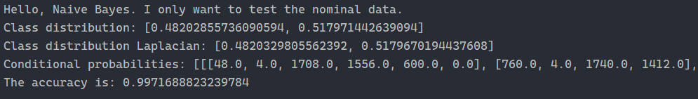
2. 运行截图

总结

优点：

(1) 算法逻辑简单, 易于实现

(2) 分类过程中时空开销小

缺点:

理论上, 朴素贝叶斯模型与其他分类方法相比具有最小的误差率. 但是实际上并非总是如此, 这是因为朴素贝叶斯模型假设属性之间相互独立, 这个假设在实际应用中往往是不成立的, 在属性个数比较多或者属性之间相关性较大时, 分类效果不好.