对同一像素点值的像素点归为一类，通过平均值进行取代，从而将图像进行压缩并且保证图像尽可能不失真，关键信息仍保留。

from PIL import Image
import numpy as np
from sklearn.cluster import KMeans
import matplotlib
import matplotlib.pyplot as plt
from mpl_toolkits.mplot3d import Axes3D


def restore_image(cb, cluster, shape):
    row, col, dummy = shape
    image = np.empty((row, col, 3))
    index = 0
    for r in range(row):
        for c in range(col):
            image[r, c] = cb[cluster[index]]
            index += 1
    return image


def show_scatter(a):
    N = 10
    print('原始数据：\n', a)
    density, edges = np.histogramdd(a, bins=[N,N,N], range=[(0,1), (0,1), (0,1)])
    density /= density.max()
    x = y = z = np.arange(N)
    d = np.meshgrid(x, y, z)

    fig = plt.figure(1, facecolor='w')
    ax = fig.add_subplot(111, projection='3d')
    ax.scatter(d[1], d[0], d[2], c='r', s=100*density, marker='o', depthshade=True)
    ax.set_xlabel(u'红色分量')
    ax.set_ylabel(u'绿色分量')
    ax.set_zlabel(u'蓝色分量')
    plt.title(u'图像颜色三维频数分布', fontsize=20)

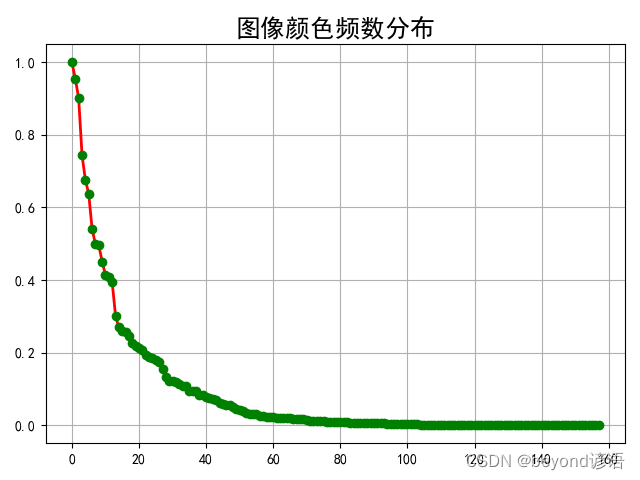
    plt.figure(2, facecolor='w')
    den = density[density > 0]
    den = np.sort(den)[::-1]
    t = np.arange(len(den))
    plt.plot(t, den, 'r-', t, den, 'go', lw=2)
    plt.title(u'图像颜色频数分布', fontsize=18)
    plt.grid(True)

    plt.show()


if __name__ == '__main__':
    matplotlib.rcParams['font.sans-serif'] = [u'SimHei']
    matplotlib.rcParams['axes.unicode_minus'] = False

    num_vq = 256 #256个像素，最后想降维到256个维度
    im = Image.open('Lena.png')     # flower2.png(200)/lena.png(50)  读取图片
    image = np.array(im).astype(np.float) / 255 # 将图像数据转化为array类型，方便后续的操作
    image = image[:, :, :3]#所有行、列、前三个维度，因为png有四个属性，RGBα，alpha为透明度，不需要，只用前三个维度信息即可
    image_v = image.reshape((-1, 3))#拉伸像素点，行不关心，列为3列===转换为二维数据，每一列均为一个维度的全部数据，RGB变成了3列，每行为一个像素点
    model = KMeans(num_vq)#通过Kmeans对每一行进行处理，也就是每个像素点进行处理，对每个像素点进行分类，像素点相似度的归类；创建聚类对象
    #每类都有一个中心像素点，将该中心像素点代替这一类，这里手动传入的是分成256个类别。不管像素点位置，只考虑相似与否是否为一类
    show_scatter(image_v)#画图

    N = image_v.shape[0]    # 图像像素总数
    # 选择足够多的样本(如1000个)，计算聚类中心
    idx = np.random.randint(0, N, size=1000)#从图像中随机选取1000个像素点
    image_sample = image_v[idx]
    model.fit(image_sample)#将这1000个像素点去训练模型，聚类结果，从1000个像素点中找到最重要的256个像素点作为中心点
    c = model.predict(image_v)  # 将图像全部的像素点进行预测，看看图像中的所有像素点离这256个簇哪一个最近，把图像的所有像素点进行分类
    print('聚类结果：\n', c)
    print('聚类中心：\n', model.cluster_centers_)

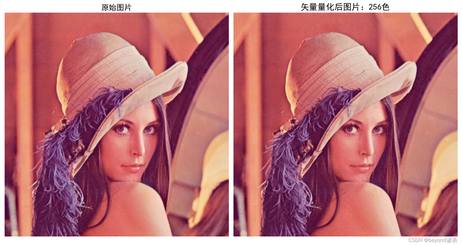
    plt.figure(figsize=(15, 8), facecolor='w')
    plt.subplot(121)
    plt.axis('off')
    plt.title(u'原始图片', fontsize=18)
    plt.imshow(image)
    #plt.savefig('1.png')

    plt.subplot(122)
    vq_image = restore_image(model.cluster_centers_, c, image.shape)#聚类中心点、聚类结果、模型图像的形状   作为参数进行恢复图像
    plt.axis('off')
    plt.title(u'矢量量化后图片：%d色' % num_vq, fontsize=20)
    plt.imshow(vq_image)
    #plt.savefig('2.png')

    plt.tight_layout()
    plt.show()