一、时间序列预测
预测可能是机器学习在现实世界中最常见的应用。 企业预测产品需求,政府预测经济和人口增长,气象学家预测天气。 对未来事物的理解是科学、政府和行业(更不用说我们的个人生活!)的迫切需求,这些领域的从业者越来越多地应用机器学习来解决这一需求。
时间序列预测是一个历史悠久的广阔领域。 本课程侧重于将现代机器学习方法应用于时间序列数据,以产生最准确的预测。 本课程中的课程受到过去 Kaggle 预测比赛中获胜解决方案的启发,但只要准确预测成为优先事项,就适用。
完成本课程后,您将知道如何:
设计功能以对主要时间序列组件(趋势、季节和周期)进行建模,
用多种时间序列图可视化时间序列,
创建结合互补模型优势的预测混合体,以及
使机器学习方法适应各种预测任务。
作为练习的一部分,您将有机会参加我们的商店销售 - 时间序列预测入门比赛。 在本次比赛中,您的任务是预测 Corporación Favorita(厄瓜多尔大型杂货零售商)近 1800 个产品类别的销售额。
Store Sales - Time Series Forecasting | KaggleUse machine learning to predict grocery sales
| 日期 | 精装书销量 |
|---|---|
| 2000-04-01 | 139 |
| 2000-04-02 | 128 |
| 2000-04-03 | 172 |
| 2000-04-04 | 139 |
| 2000-04-05 | 191 |
上表记录了一家零售店 30 天内精装书的销售数量。 请注意,我们有一列带有时间索引日期的精装观察。
二、具有时间序列的线性回归
在本课程的第一部分,我们将使用线性回归算法来构建预测模型。 线性回归在实践中被广泛使用,并且自然地适应甚至复杂的预测任务。
线性回归算法学习如何从其输入特征中得出加权和。 对于两个功能,我们将拥有:
target = weight_1 * feature_1 + weight_2 * feature_2 + bias在训练期间,回归算法学习参数 weight_1、weight_2 和最适合目标的偏差的值。 (该算法通常被称为普通最小二乘法,因为它选择的值可以使目标和预测之间的平方误差最小化。)权重也称为回归系数,偏差也称为截距,因为它说明了位置函数穿过 y 轴。
1、时间步长特征
时间序列有两种独特的特征:时间步长特征和滞后特征。
时间步长特征是我们可以直接从时间索引中得出的特征。 最基本的时间步长特征是时间虚拟变量,它从头到尾计算序列中的时间步长。
import numpy as np
df['Time'] = np.arange(len(df.index))
df.head()| Date | Hardcover | Time |
|---|---|---|
| 2000-04-01 | 139 | 0 |
| 2000-04-02 | 128 | 1 |
| 2000-04-03 | 172 | 2 |
| 2000-04-04 | 139 | 3 |
| 2000-04-05 | 191 | 4 |
具有时间虚拟变量的线性回归产生模型:
target = weight * time + bias然后,时间虚拟变量让我们将曲线拟合到时间图中的时间序列,其中时间形成 x 轴。
import matplotlib.pyplot as plt
import seaborn as sns
plt.style.use("seaborn-whitegrid")
plt.rc(
    "figure",
    autolayout=True,
    figsize=(11, 4),
    titlesize=18,
    titleweight='bold',
)
plt.rc(
    "axes",
    labelweight="bold",
    labelsize="large",
    titleweight="bold",
    titlesize=16,
    titlepad=10,
)
%config InlineBackend.figure_format = 'retina'

fig, ax = plt.subplots()
ax.plot('Time', 'Hardcover', data=df, color='0.75')
ax = sns.regplot(x='Time', y='Hardcover', data=df, ci=None, scatter_kws=dict(color='0.25'))
ax.set_title('Time Plot of Hardcover Sales');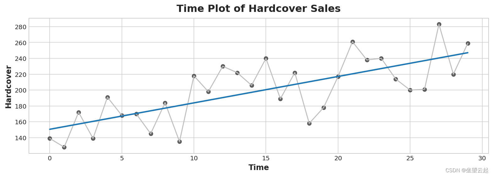
时间步长功能可让您对时间依赖性进行建模。 如果一个系列的值可以从它们发生的时间预测出来,那么它就是时间相关的。 在精装销售系列中,我们可以预测当月晚些时候的销售量通常高于本月早些时候的销售量。
2、滞后特征
为了制作滞后特征,我们改变了目标系列的观察结果,使它们看起来发生在较晚的时间。 在这里,我们创建了一个 1 步滞后功能,尽管也可以进行多步移动。
df['Lag_1'] = df['Hardcover'].shift(1)
df = df.reindex(columns=['Hardcover', 'Lag_1'])
df.head()| Date | Hardcover | Lag_1 |
|---|---|---|
| 2000-04-01 | 139 | NaN |
| 2000-04-02 | 128 | 139.0 |
| 2000-04-03 | 172 | 128.0 |
| 2000-04-04 | 139 | 172.0 |
| 2000-04-05 | 191 | 139.0 |
具有滞后特征的线性回归产生模型:
target = weight * lag + bias因此,滞后特征让我们可以将曲线拟合到滞后图中,其中系列中的每个观察值都与前一个观察值相对应。
fig, ax = plt.subplots()
ax = sns.regplot(x='Lag_1', y='Hardcover', data=df, ci=None, scatter_kws=dict(color='0.25'))
ax.set_aspect('equal')
ax.set_title('Lag Plot of Hardcover Sales');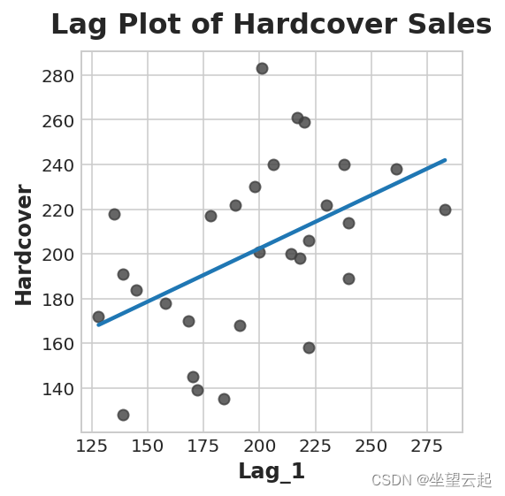
您可以从滞后图中看到,某一天的销售额(精装本)与前一天的销售额(Lag_1)相关。 当您看到这样的关系时,您就会知道延迟功能会很有用。
更一般地说,滞后功能可以让您对串行依赖进行建模。 当可以从先前的观察中预测观察时,时间序列具有序列依赖性。 在精装销售中,我们可以预测一天的高销售额通常意味着第二天的高销售额。
使机器学习算法适应时间序列问题主要是关于具有时间索引和滞后的特征工程。对于大部分课程,我们使用线性回归是为了简单,但无论您为预测任务选择哪种算法,这些功能都会很有用。
三、示例 - 隧道流量
Tunnel Traffic 是一个时间序列,描述了从 2003 年 11 月到 2005 年 11 月期间每天通过瑞士巴雷格隧道的车辆数量。在这个例子中,我们将进行一些练习,将线性回归应用于时间步长特征和滞后特征。
隐藏的单元格设置了所有内容。
from pathlib import Path
from warnings import simplefilter

import matplotlib.pyplot as plt
import numpy as np
import pandas as pd

simplefilter("ignore")  # ignore warnings to clean up output cells

# Set Matplotlib defaults
plt.style.use("seaborn-whitegrid")
plt.rc("figure", autolayout=True, figsize=(11, 4))
plt.rc(
    "axes",
    labelweight="bold",
    labelsize="large",
    titleweight="bold",
    titlesize=14,
    titlepad=10,
)
plot_params = dict(
    color="0.75",
    style=".-",
    markeredgecolor="0.25",
    markerfacecolor="0.25",
    legend=False,
)
%config InlineBackend.figure_format = 'retina'


# Load Tunnel Traffic dataset
data_dir = Path("../input/ts-course-data")
tunnel = pd.read_csv(data_dir / "tunnel.csv", parse_dates=["Day"])

# Create a time series in Pandas by setting the index to a date
# column. We parsed "Day" as a date type by using `parse_dates` when
# loading the data.
tunnel = tunnel.set_index("Day")

# By default, Pandas creates a `DatetimeIndex` with dtype `Timestamp`
# (equivalent to `np.datetime64`, representing a time series as a
# sequence of measurements taken at single moments. A `PeriodIndex`,
# on the other hand, represents a time series as a sequence of
# quantities accumulated over periods of time. Periods are often
# easier to work with, so that's what we'll use in this course.
tunnel = tunnel.to_period()

tunnel.head()| Day | NumVehicles |
|---|---|
| 2003-11-01 | 103536 |
| 2003-11-02 | 92051 |
| 2003-11-03 | 100795 |
| 2003-11-04 | 102352 |
| 2003-11-05 | 106569 |
1、时间步长特征
如果时间序列没有任何缺失的日期,我们可以通过计算序列的长度来创建时间虚拟对象。
df = tunnel.copy()
df['Time'] = np.arange(len(tunnel.index))
df.head()| Day | NumVehicles | Time |
|---|---|---|
| 2003-11-01 | 103536 | 0 |
| 2003-11-02 | 92051 | 1 |
| 2003-11-03 | 100795 | 2 |
| 2003-11-04 | 102352 | 3 |
| 2003-11-05 | 106569 | 4 |
拟合线性回归模型的过程遵循 scikit-learn 的标准步骤。
from sklearn.linear_model import LinearRegression

# Training data
X = df.loc[:, ['Time']]  # features
y = df.loc[:, 'NumVehicles']  # target

# Train the model
model = LinearRegression()
model.fit(X, y)

# Store the fitted values as a time series with the same time index as
# the training data
y_pred = pd.Series(model.predict(X), index=X.index)
实际创建的模型(大约)为:Vehicles = 22.5 * Time + 98176。绘制随时间变化的拟合值向我们展示了如何将线性回归拟合到时间虚拟变量创建由该方程定义的趋势线。
ax = y.plot(**plot_params)
ax = y_pred.plot(ax=ax, linewidth=3)
ax.set_title('Time Plot of Tunnel Traffic');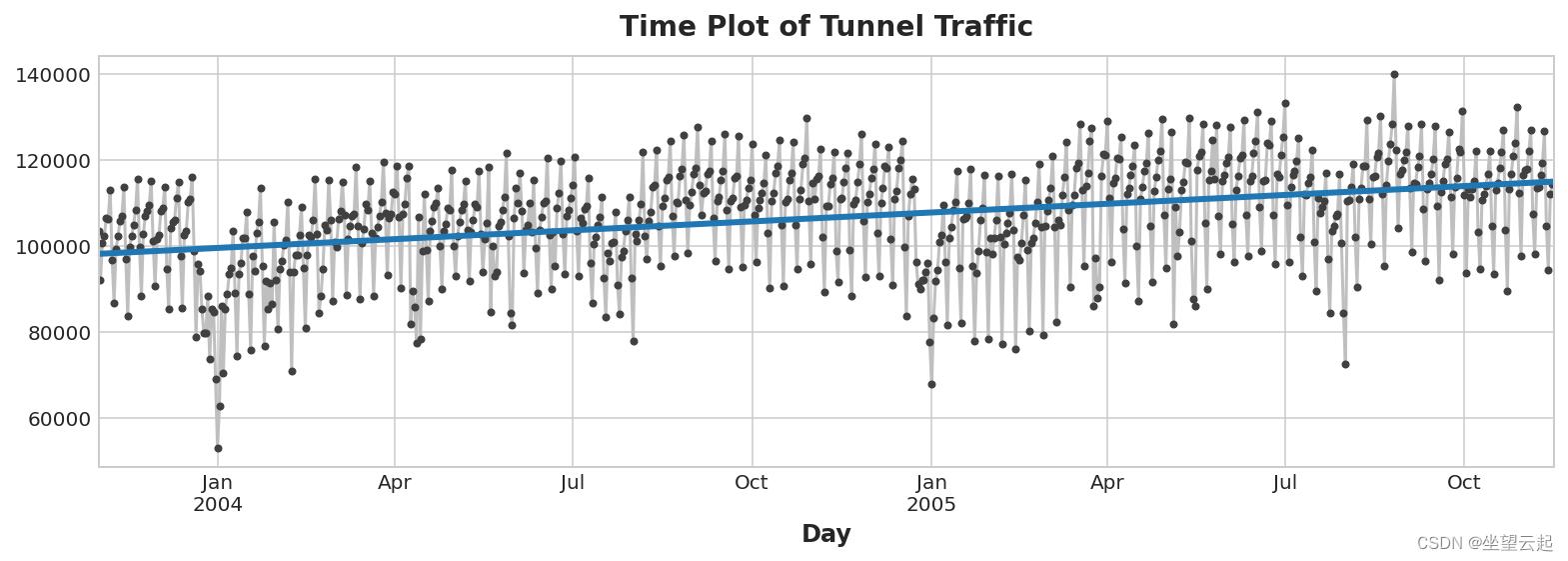
2、滞后特征
Pandas 为我们提供了一种简单的滞后序列的方法,即 shift 方法。
df['Lag_1'] = df['NumVehicles'].shift(1)
df.head()| Day | NumVehicles | Time | Lag_1 |
|---|---|---|---|
| 2003-11-01 | 103536 | 0 | NaN |
| 2003-11-02 | 92051 | 1 | 103536.0 |
| 2003-11-03 | 100795 | 2 | 92051.0 |
| 2003-11-04 | 102352 | 3 | 100795.0 |
| 2003-11-05 | 106569 | 4 | 102352.0 |
创建滞后特征时,我们需要决定如何处理产生的缺失值。 填充它们是一种选择,可能使用 0.0 或使用第一个已知值“回填”。 相反,我们将只删除缺失的值,并确保从相应日期删除目标中的值。
from sklearn.linear_model import LinearRegression

X = df.loc[:, ['Lag_1']]
X.dropna(inplace=True)  # drop missing values in the feature set
y = df.loc[:, 'NumVehicles']  # create the target
y, X = y.align(X, join='inner')  # drop corresponding values in target

model = LinearRegression()
model.fit(X, y)

y_pred = pd.Series(model.predict(X), index=X.index)
滞后图向我们展示了我们能够很好地拟合一天车辆数量与前一天车辆数量之间的关系。
fig, ax = plt.subplots()
ax.plot(X['Lag_1'], y, '.', color='0.25')
ax.plot(X['Lag_1'], y_pred)
ax.set_aspect('equal')
ax.set_ylabel('NumVehicles')
ax.set_xlabel('Lag_1')
ax.set_title('Lag Plot of Tunnel Traffic');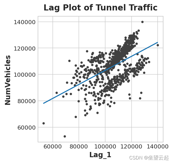
这个来自滞后特征的预测意味着我们可以在多大程度上预测跨时间的序列? 下面的时间图向我们展示了我们的预测现在如何响应该系列最近的行为。
ax = y.plot(**plot_params)
ax = y_pred.plot()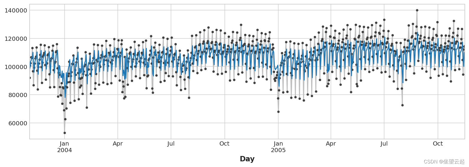
最好的时间序列模型通常会包含一些时间步长特征和滞后特征的组合。 在接下来的几节课中,我们将学习如何使用本课中的特征作为起点,对时间序列中最常见的模式进行建模。
继续练习,您将开始使用您在本教程中学到的技术来预测商店销售额。