《MATLAB智能算法30个案例》:第15章 基于混合粒子群算法的TSP搜索算法
1. 前言
《MATLAB智能算法30个案例分析》是2011年7月1日由北京航空航天大学出版社出版的图书,作者是郁磊、史峰、王辉、胡斐。本书案例是各位作者多年从事算法研究的经验总结。书中所有案例均因国内各大MATLAB技术论坛网友的切身需求而精心设计,其中不少案例所涉及的内容和求解方法在国内现已出版的MATLAB书籍中鲜有介绍。《MATLAB智能算法30个案例分析》采用案例形式,以智能算法为主线,讲解了遗传算法、免疫算法、退火算法、粒子群算法、鱼群算法、蚁群算法和神经网络算法等最常用的智能算法的MATLAB实现。
本书共给出30个案例,每个案例都是一个使用智能算法解决问题的具体实例,所有案例均由理论讲解、案例背景、MATLAB程序实现和扩展阅读四个部分组成,并配有完整的原创程序,使读者在掌握算法的同时更能快速提高使用算法求解实际问题的能力。《MATLAB智能算法30个案例分析》可作为本科毕业设计、研究生项目设计、博士低年级课题设计参考书籍,同时对广大科研人员也有很高的参考价值。
《MATLAB智能算法30个案例分析》与《MATLAB 神经网络43个案例分析》一样,都是由北京航空航天大学出版社出版,其中的智能算法应该是属于神经网络兴起之前的智能预测分类算法的热门领域,在数字信号处理,如图像和语音相关方面应用较为广泛。本系列文章结合MATLAB与实际案例进行仿真复现,有不少自己在研究生期间与工作后的学习中有过相关学习应用,这次复现仿真示例进行学习,希望可以温故知新,加强并提升自己在智能算法方面的理解与实践。下面开始进行仿真示例,主要以介绍各章节中源码应用示例为主,本文主要基于MATLAB2015b(32位)平台仿真实现,这是本书第十五章基于混合粒子群算法的TSP搜索算法实例,话不多说,开始!
2. MATLAB 仿真示例
打开MATLAB,点击“主页”,点击“打开”,找到示例文件
选中main.m,点击“打开”
main.m源码如下:
%%%%%%%%%%%%%%%%%%%%%%%%%%%%%%%%%%%%%%%%%%%%%%%%%%%%
%功能:基于TSP-PSO算法示例
%环境:Win7,Matlab2015b
%Modi: C.S
%时间:2022-07-08
%%%%%%%%%%%%%%%%%%%%%%%%%%%%%%%%%%%%%%%%%%%%%%%%%%%%
%% 清空环境
clc
clear all
close all
tic
%% 下载数据
data=load('eil51.txt');
cityCoor=[data(:,2) data(:,3)];%城市坐标矩阵
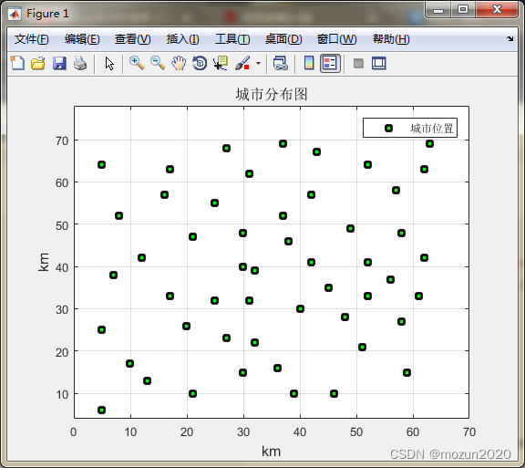
figure
plot(cityCoor(:,1),cityCoor(:,2),'ms','LineWidth',2,'MarkerEdgeColor','k','MarkerFaceColor','g')
legend('城市位置')
ylim([4 78])
title('城市分布图','fontsize',12)
xlabel('km','fontsize',12)
ylabel('km','fontsize',12)
%ylim([min(cityCoor(:,2))-1 max(cityCoor(:,2))+1])
grid on
%% 计算城市间距离
n=size(cityCoor,1); %城市数目
cityDist=zeros(n,n); %城市距离矩阵
for i=1:n
for j=1:n
if i~=j
cityDist(i,j)=((cityCoor(i,1)-cityCoor(j,1))^2+...
(cityCoor(i,2)-cityCoor(j,2))^2)^0.5;
end
cityDist(j,i)=cityDist(i,j);
end
end
nMax=200; %进化次数
indiNumber=1000; %个体数目
individual=zeros(indiNumber,n);
%^初始化粒子位置
for i=1:indiNumber
individual(i,:)=randperm(n);
end
%% 计算种群适应度
indiFit=fitness(individual,cityCoor,cityDist);
[value,index]=min(indiFit);
tourPbest=individual; %当前个体最优
tourGbest=individual(index,:) ; %当前全局最优
recordPbest=inf*ones(1,indiNumber); %个体最优记录
recordGbest=indiFit(index); %群体最优记录
xnew1=individual;
%% 循环寻找最优路径
L_best=zeros(1,nMax);
for N=1:nMax
N
%计算适应度值
indiFit=fitness(individual,cityCoor,cityDist);
%更新当前最优和历史最优
for i=1:indiNumber
if indiFit(i)<recordPbest(i)
recordPbest(i)=indiFit(i);
tourPbest(i,:)=individual(i,:);
end
if indiFit(i)<recordGbest
recordGbest=indiFit(i);
tourGbest=individual(i,:);
end
end
[value,index]=min(recordPbest);
recordGbest(N)=recordPbest(index);
%% 交叉操作
for i=1:indiNumber
% 与个体最优进行交叉
c1=unidrnd(n-1); %产生交叉位
c2=unidrnd(n-1); %产生交叉位
while c1==c2
c1=round(rand*(n-2))+1;
c2=round(rand*(n-2))+1;
end
chb1=min(c1,c2);
chb2=max(c1,c2);
cros=tourPbest(i,chb1:chb2);
ncros=size(cros,2);
%删除与交叉区域相同元素
for j=1:ncros
for k=1:n
if xnew1(i,k)==cros(j)
xnew1(i,k)=0;
for t=1:n-k
temp=xnew1(i,k+t-1);
xnew1(i,k+t-1)=xnew1(i,k+t);
xnew1(i,k+t)=temp;
end
end
end
end
%插入交叉区域
xnew1(i,n-ncros+1:n)=cros;
%新路径长度变短则接受
dist=0;
for j=1:n-1
dist=dist+cityDist(xnew1(i,j),xnew1(i,j+1));
end
dist=dist+cityDist(xnew1(i,1),xnew1(i,n));
if indiFit(i)>dist
individual(i,:)=xnew1(i,:);
end
% 与全体最优进行交叉
c1=round(rand*(n-2))+1; %产生交叉位
c2=round(rand*(n-2))+1; %产生交叉位
while c1==c2
c1=round(rand*(n-2))+1;
c2=round(rand*(n-2))+1;
end
chb1=min(c1,c2);
chb2=max(c1,c2);
cros=tourGbest(chb1:chb2);
ncros=size(cros,2);
%删除与交叉区域相同元素
for j=1:ncros
for k=1:n
if xnew1(i,k)==cros(j)
xnew1(i,k)=0;
for t=1:n-k
temp=xnew1(i,k+t-1);
xnew1(i,k+t-1)=xnew1(i,k+t);
xnew1(i,k+t)=temp;
end
end
end
end
%插入交叉区域
xnew1(i,n-ncros+1:n)=cros;
%新路径长度变短则接受
dist=0;
for j=1:n-1
dist=dist+cityDist(xnew1(i,j),xnew1(i,j+1));
end
dist=dist+cityDist(xnew1(i,1),xnew1(i,n));
if indiFit(i)>dist
individual(i,:)=xnew1(i,:);
end
%% 变异操作
c1=round(rand*(n-1))+1; %产生变异位
c2=round(rand*(n-1))+1; %产生变异位
while c1==c2
c1=round(rand*(n-2))+1;
c2=round(rand*(n-2))+1;
end
temp=xnew1(i,c1);
xnew1(i,c1)=xnew1(i,c2);
xnew1(i,c2)=temp;
%新路径长度变短则接受
dist=0;
for j=1:n-1
dist=dist+cityDist(xnew1(i,j),xnew1(i,j+1));
end
dist=dist+cityDist(xnew1(i,1),xnew1(i,n));
if indiFit(i)>dist
individual(i,:)=xnew1(i,:);
end
end
[value,index]=min(indiFit);
L_best(N)=indiFit(index);
tourGbest=individual(index,:);
end
%% 结果作图
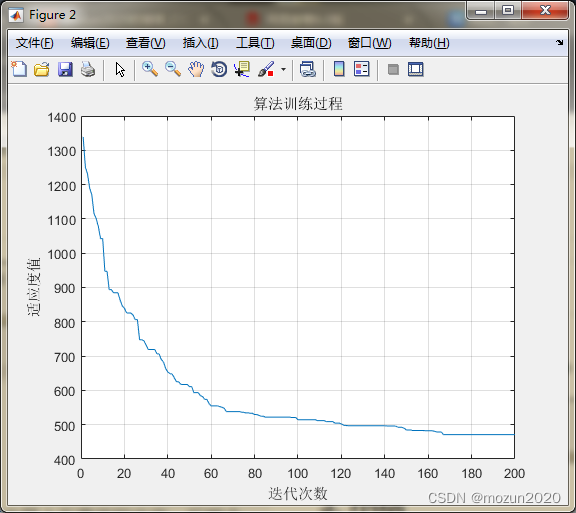
figure
plot(L_best)
title('算法训练过程')
xlabel('迭代次数')
ylabel('适应度值')
grid on
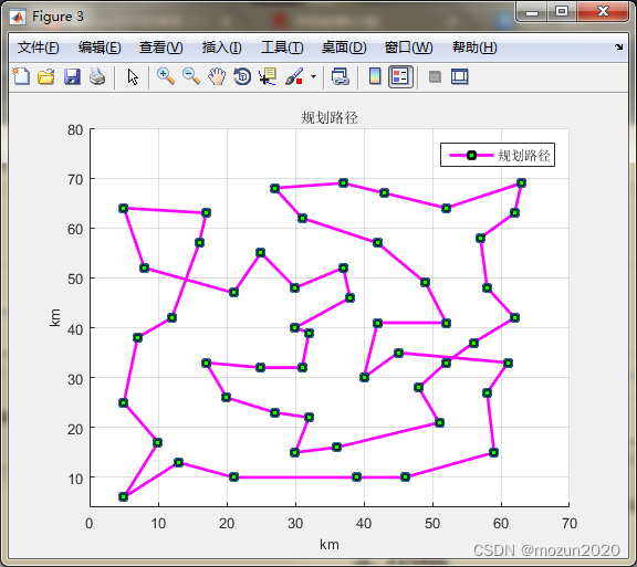
figure
hold on
plot([cityCoor(tourGbest(1),1),cityCoor(tourGbest(n),1)],[cityCoor(tourGbest(1),2),...
cityCoor(tourGbest(n),2)],'ms-','LineWidth',2,'MarkerEdgeColor','k','MarkerFaceColor','g')
hold on
for i=2:n
plot([cityCoor(tourGbest(i-1),1),cityCoor(tourGbest(i),1)],[cityCoor(tourGbest(i-1),2),...
cityCoor(tourGbest(i),2)],'ms-','LineWidth',2,'MarkerEdgeColor','k','MarkerFaceColor','g')
hold on
end
legend('规划路径')
scatter(cityCoor(:,1),cityCoor(:,2));
title('规划路径','fontsize',10)
xlabel('km','fontsize',10)
ylabel('km','fontsize',10)
grid on
ylim([4 80])
toc
添加完毕,点击“运行”,开始仿真,输出仿真结果如下:
N =

     1


N =

     2


N =

     3


N =

     4


N =

     5


N =

     6


N =

     7


N =

     8


N =

     9


N =

    10


N =

    11


N =

    12


N =

    13


N =

    14


N =

    15


N =

    16


N =

    17


N =

    18


N =

    19


N =

    20


N =

    21


N =

    22


N =

    23


N =

    24


N =

    25


N =

    26


N =

    27


N =

    28


N =

    29


N =

    30


N =

    31


N =

    32


N =

    33


N =

    34


N =

    35


N =

    36


N =

    37


N =

    38


N =

    39


N =

    40


N =

    41


N =

    42


N =

    43


N =

    44


N =

    45


N =

    46


N =

    47


N =

    48


N =

    49


N =

    50


N =

    51


N =

    52


N =

    53


N =

    54


N =

    55


N =

    56


N =

    57


N =

    58


N =

    59


N =

    60


N =

    61


N =

    62


N =

    63


N =

    64


N =

    65


N =

    66


N =

    67


N =

    68


N =

    69


N =

    70


N =

    71


N =

    72


N =

    73


N =

    74


N =

    75


N =

    76


N =

    77


N =

    78


N =

    79


N =

    80


N =

    81


N =

    82


N =

    83


N =

    84


N =

    85


N =

    86


N =

    87


N =

    88


N =

    89


N =

    90


N =

    91


N =

    92


N =

    93


N =

    94


N =

    95


N =

    96


N =

    97


N =

    98


N =

    99


N =

   100


N =

   101


N =

   102


N =

   103


N =

   104


N =

   105


N =

   106


N =

   107


N =

   108


N =

   109


N =

   110


N =

   111


N =

   112


N =

   113


N =

   114


N =

   115


N =

   116


N =

   117


N =

   118


N =

   119


N =

   120


N =

   121


N =

   122


N =

   123


N =

   124


N =

   125


N =

   126


N =

   127


N =

   128


N =

   129


N =

   130


N =

   131


N =

   132


N =

   133


N =

   134


N =

   135


N =

   136


N =

   137


N =

   138


N =

   139


N =

   140


N =

   141


N =

   142


N =

   143


N =

   144


N =

   145


N =

   146


N =

   147


N =

   148


N =

   149


N =

   150


N =

   151


N =

   152


N =

   153


N =

   154


N =

   155


N =

   156


N =

   157


N =

   158


N =

   159


N =

   160


N =

   161


N =

   162


N =

   163


N =

   164


N =

   165


N =

   166


N =

   167


N =

   168


N =

   169


N =

   170


N =

   171


N =

   172


N =

   173


N =

   174


N =

   175


N =

   176


N =

   177


N =

   178


N =

   179


N =

   180


N =

   181


N =

   182


N =

   183


N =

   184


N =

   185


N =

   186


N =

   187


N =

   188


N =

   189


N =

   190


N =

   191


N =

   192


N =

   193


N =

   194


N =

   195


N =

   196


N =

   197


N =

   198


N =

   199


N =

   200

时间已过 53.366828 秒。
3. 小结
最初的PSO算法是用来解决连续空间问题的, 为了适合求解离散域TSP问题, 人们对算法进行了各种改进。结合遗传算法和模拟退火算法的思想, 有学者提出用混合粒子群算法来求解 TSP问题,关于TSP问题的仿真示例,在其他方法张红也有相关示例,链接见文末。对本章内容感兴趣或者想充分学习了解的,建议去研习书中第十五章节的内容。后期会对其中一些知识点在自己理解的基础上进行补充,欢迎大家一起学习交流。