上一篇文章GC-LSTM原理部分中具体介绍了GC-LSTM的原理，这里基于PyG Temporal中的GCLSTM模块对实现一个基于GC-LSTM的预测模型。注：这里可以是流量预测等各种节点特征。

一、数据预处理

这里图拓扑的结构和邻接矩阵如图所示，：

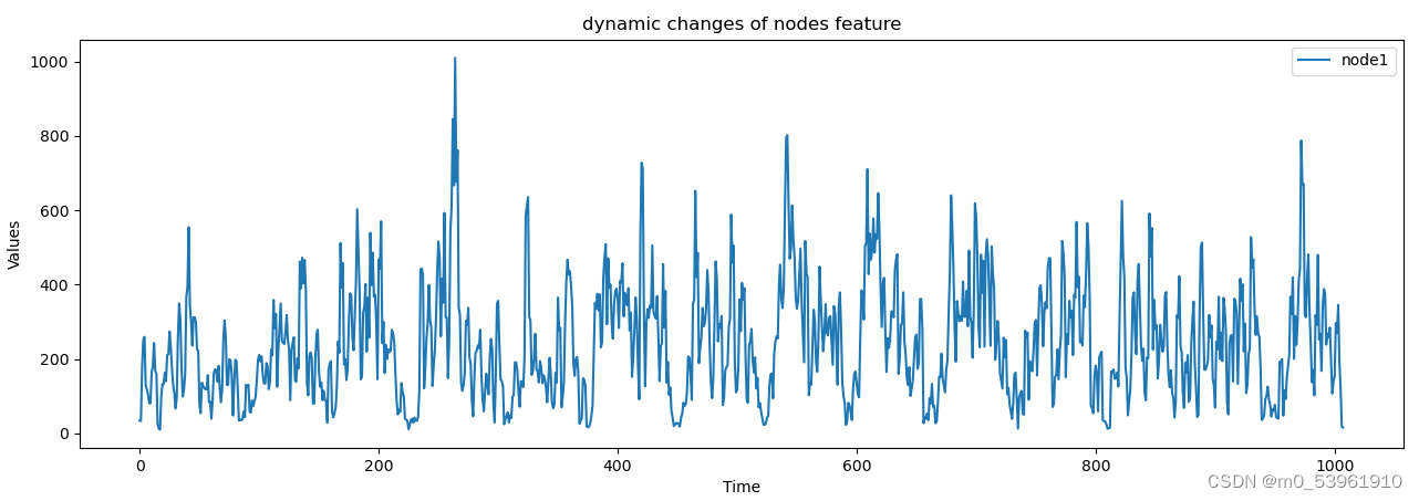
节点特征矩阵，这里只展示了其中一个节点的特征向量随时间的变化，只选取了一个指标即：

 接下来我们需要对数据进行预处理，具体过程如代码所示：

def clean_train_test_data(traindata, testdata):
    sc = MinMaxScaler(feature_range = (-1, 1))
    # sc = StandardScaler()
    train_data= sc.fit_transform(traindata)
    test_data = sc.transform(testdata)  # 利用训练集的属性对测试集进行归一化
    return train_data, test_data


# 将数据划分为训练集与测试集,前80%的数据作为训练集，后20%的数据作为测试集
train_size = int(len(node_cpu)*0.8)
test_size = len(node_cpu) - train_size
train_data = node_cpu[0:train_size, :]
test_data = node_cpu[train_size:len(node_cpu), :]
train_data, test_data = clean_train_test_data(train_data, test_data)
# print(train_data.shape)(806, 10)
# print(test_data.shape)(202, 10)
train_data = np.array(train_data).transpose()
test_data = np.array(test_data).transpose()
# print(train_data.shape)#(10, 806)
def split_dataset(data, n_sequence, n_pre):
    '''
    对数据进行处理，根据输入模型的历史数据长度和预测数据长度对数据进行切分
    :param data: 输入数据集
    :param n_sequence: 历史数据长度
    :param n_pre: 预测数据长度
    :return: 划分好的train data和target data
    '''
    train_X, train_Y = [], []
    for i in range(data.shape[1] - n_sequence - n_pre):
        a = data[:, i:(i + n_sequence)]
        train_X.append(a)
        b = data[:, (i + n_sequence):(i + n_sequence + n_pre)]
        train_Y.append(b)

    # train_X = np.array(train_X)
    # train_Y = np.array(train_Y)

    return train_X, train_Y

history_data = 72
predict_data = 1
train_feature, train_target = split_dataset(train_data, history_data, predict_data)
test_feature, test_target = split_dataset(test_data, history_data, predict_data)
# print(train_feature.shape, train_target.shape)#(733, 10, 72) (733, 10, 1)
# print(test_feature.shape, test_target.shape)#(129, 10, 72) (129, 10, 1)
# 数据的邻接矩阵A
edge_index = np.array([[0, 1, 0, 2, 0, 3, 0, 4, 0, 5, 0, 7, 1, 2, 1, 6, 2, 3, 2, 8, 2, 9, 3, 4, 3, 5, 3, 6, 3, 7, 5, 9, 7, 8],
                       [1, 0, 2, 0, 3, 0, 4, 0, 5, 0, 7, 0, 2, 1, 6, 1, 3, 2, 8, 2, 9, 2, 4, 3, 5, 3, 6, 3, 7, 3, 9, 5, 8, 7]])
'''PyG Temporal中的类似DataLoader的数据处理器：
    edge_index：是邻接矩阵；
    edge_weight：是每个链路的权重；
    features：是输入历史节点特征矩阵；
    targets：是输入预测节点特征举证ground-truth；'''
train_dataset = StaticGraphTemporalSignal(edge_index=edge_index, edge_weight=np.ones(edge_index.shape[1]), features=train_feature, targets=train_target)
test_dataset = StaticGraphTemporalSignal(edge_index=edge_index, edge_weight=np.ones(edge_index.shape[1]), features=test_feature, targets=test_target)
# print("Number of train buckets: ", len(set(train_dataset)))#733
# print("Number of test buckets: ", len(set(test_dataset)))#129

二、模型

这里是模型部分的代码，关于GCN的详细介绍和实现，GCN从0到1里面以及说的很详细了，这里不在过多赘述；关于GCN-LSTM模型的介绍，在这里。这里需要说明的一点是，GCN_LSTM中的input_size其实是数据经过GCN处理之后的output_size，也就是输入到LSTM中的input_size。

class GCN_LSTM(torch.nn.Module):
    def __init__(self, node_features, input_size, output_size):
        super(GCN_LSTM, self).__init__()
        self.recurrent = GCLSTM(node_features, input_size, output_size)
        self.MLP = torch.nn.Sequential(
            torch.nn.Linear(input_size, input_size // 2),
            torch.nn.ReLU(inplace=True),
            torch.nn.Linear(input_size // 2, input_size // 4),
            torch.nn.ReLU(inplace=True),
            torch.nn.Linear(input_size // 4, output_size))


    def forward(self, x, edge_index, edge_weight):
        x, _ = self.recurrent(x, edge_index, edge_weight)
        x = F.relu(x)
        x = F.dropout(x, training=self.training)
        x = self.MLP(x)
        return x


model = GCN_LSTM(node_features=72, input_size=36, output_size=1)
optimizer = torch.optim.Adam(model.parameters(), lr=0.01, weight_decay=1.5e-3)
loss_mse = torch.nn.MSELoss()
cost_list = []
model.train()
'''time为train size'''
for epoch in tqdm(range(300)):
    cost = 0
    for time, snapshot in enumerate(train_dataset):
        y_hat = model(snapshot.x, snapshot.edge_index, snapshot.edge_attr)
        cost = cost + loss_mse(y_hat, snapshot.y)
    cost = cost / (time + 1)
    cost_list.append(cost.item())
    cost.backward()
    optimizer.step()
    optimizer.zero_grad()
cost = cost.item()
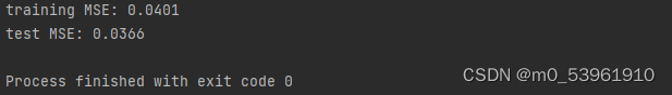
print("training MSE: {:.4f}".format(cost))

plt.plot(cost_list)
plt.xlabel("Epoch")
plt.ylabel("MSE")
plt.title("average of Training cost for 10 nodes")
plt.show()

model.eval()
cost = 0
test_real = []
test_pre = []
cha = []
for time, snapshot in enumerate(test_dataset):
    y_hat = model(snapshot.x, snapshot.edge_index, snapshot.edge_attr)
    test_pre.append(y_hat.detach().numpy())
    test_real.append(snapshot.y.detach().numpy())
    cost = cost + torch.mean((y_hat - snapshot.y) ** 2)
    cha_node = y_hat - snapshot.y
    cha.append(cha_node.detach().numpy())
    # print('cost', cost)
    # print('cha', cha_node)
cost = cost / (time + 1)
cost = cost.item()
print("test MSE: {:.4f}".format(cost))
test_real = np.array(test_real)
test_real = test_real.reshape([test_real.shape[0], test_real.shape[2]])
test_pre = np.array(test_pre)
test_pre = test_pre.reshape([test_pre.shape[0], test_pre.shape[2]])

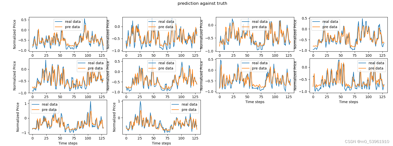
plt.figure(1)
for i in range(test_real.shape[1]):
    plt.subplot(3, 4, 1+i)
    plt.plot(test_real[:, i], label='real data')
    plt.plot(test_pre[:, i], label='pre data')
    plt.xlabel("Time steps")
    plt.ylabel("Normalized Price")
    plt.suptitle("prediction against truth")
    plt.legend()
plt.show()

输出结果

损失函数：

预测结果：