前言
本文介绍循环神经网络的进阶案例,通过搭建和训练一个模型,来对钢琴的音符进行预测,通过重复调用模型来进而生成一段音乐;
使用到Maestro的钢琴MIDI文件 ,每个文件由不同音符组成,音符用三个量来表示:音高pitch、步长step、持续时间duration。通过搭建和训练循环神经网络模型,输入一系列音符能预测下一个音符。
下图是一个钢琴MIDI文件,由不同音符组成:
思路流程
- 导入数据集
- 探索集数据,并进行数据预处理
- 构建模型(搭建神经网络结构、编译模型)
- 训练模型(把数据输入模型、评估准确性、作出预测、验证预测)
- 使用训练好的模型
- 优化模型、重新构建模型、训练模型、使用模型
一、导入数据集
使用到Maestro的钢琴MIDI文件 ,每个文件中由不同音轨组成,音轨中包含了一些音符;我们可以通过遍历每个音轨中的音符,获取音符的开始时间、结束时间、音高、音量等信息,进行音乐分析和处理。
我们到Maestro下载maestro-v2.0.0-midi.zip文件,它包含1282个钢琴MIDI文件,大约58M左右;解压后能看到如下的文件。
2004
2006
2008
2009
扫描二维码关注公众号,回复: 14610290 查看本文章
2011
2013
2014
2015
2017
2018
LICENSE
maestro-v2.0.0.csv
maestro-v2.0.0.json
README
我们可以使用电脑播放器打开文件夹中钢琴MIDI文件,比如:maestro-v2.0.0/2004/MIDI-Unprocessed_SMF_02_R1_2004_01-05_ORIG_MID--AUDIO_02_R1_2004_05_Track05_wav.midi文件,能听到一段钢琴音乐。
二、探索集数据,并进行数据预处理
2.1 解析MIDI文件
我们使用 pretty_midi 库创建和解析MIDI文件,首先安装一下它,执行如下的命令:
!pip install pretty_midi在notebook jupytre中播放MIDI音频文件,需要安装pyfluidsynth库,执行如下的命令:
!sudo apt install -y fluidsynth写一个程序解析MIDI文件,
import glob
import pretty_midi


# 加载maestro-v2.0.0目录下的每个midi文件
filenames = glob.glob(str('./maestro-v2.0.0/*/*.mid*'))
print('Number of files:', len(filenames))

# 使用pretty_midi库解析单个MIDI文件,并检查音符的格式
sample_file = filenames[1]
print(sample_file)
pm = pretty_midi.PrettyMIDI(sample_file)

# 对MIDI文件进行检查
print('Number of instruments:', len(pm.instruments))
instrument = pm.instruments[0]
instrument_name = pretty_midi.program_to_instrument_name(instrument.program)
print('Instrument name:', instrument_name)
2.2 提取音符
在训练模型时,将使用三个变量来表示音符:pitch、step 和 duration。
- pitch是音符的音高,以MIDI音高值表示,范围是0到127,0表示最低音高,127表示最高音高。
- step是是从上一个音符或曲目的开始经过的时间。
- duration是音符的持续时间,以“ticks”为单位表示,一个tick表示MIDI时间分辨率中的最小时间单位,具体的时间取决于MIDI文件的时间分辨率参数。
所以我们需要对每个MIDI文件进行提取音符。
上面打开的xxxMIDI文件,查看它的5个音符
# 查看xxxMIDI文件的10个音符
for i, note in enumerate(instrument.notes[:5]):
  note_name = pretty_midi.note_number_to_name(note.pitch)
  duration = note.end - note.start
  print(f'{i}: pitch={note.pitch}, note_name={note_name},'
        f' duration={duration:.4f}')
能看到如下的信息
0: pitch=78, note_name=F#5, duration=0.0292
1: pitch=66, note_name=F#4, duration=0.0333
2: pitch=71, note_name=B4, duration=0.0292
3: pitch=83, note_name=B5, duration=0.0365
4: pitch=73, note_name=C#5, duration=0.0333
写一个函数来从MIDI文件中提取音符
import pandas as pd
import collections
import numpy as np

# 从MIDI文件中提取音符
def midi_to_notes(midi_file: str) -> pd.DataFrame:
  pm = pretty_midi.PrettyMIDI(midi_file)
  instrument = pm.instruments[0]
  notes = collections.defaultdict(list)

  # 按开始时间对笔记排序
  sorted_notes = sorted(instrument.notes, key=lambda note: note.start)
  prev_start = sorted_notes[0].start

  for note in sorted_notes:
    start = note.start
    end = note.end
    notes['pitch'].append(note.pitch)
    notes['start'].append(start)
    notes['end'].append(end)
    notes['step'].append(start - prev_start)
    notes['duration'].append(end - start)
    prev_start = start

  return pd.DataFrame({name: np.array(value) for name, value in notes.items()})
通过midi_to_notes函数,提取一个MIDI文件中提取音符
raw_notes = midi_to_notes('./xxx.midi')
raw_notes.head()
比如,MIDI文件名称为:maestro-v2.0.0/2004/MIDI-Unprocessed_XP_14_R1_2004_01-03_ORIG_MID--AUDIO_14_R1_2004_03_Track03_wav.midi
pitch是音高。duration 是音符将播放多长时间(以秒为单位),是音符结束时间(end)和音符开始时间(start)之间的差值。step 是从前一个音符开始所经过的时间。
| pitch | start | end | step | duration | |
|---|---|---|---|---|---|
| 0 | 78 | 1.066667 | 1.095833 | 0.000000 | 0.029167 |
| 1 | 66 | 1.071875 | 1.105208 | 0.005208 | 0.033333 |
| 2 | 83 | 1.217708 | 1.254167 | 0.145833 | 0.036458 |
| 3 | 71 | 1.220833 | 1.250000 | 0.003125 | 0.029167 |
| 4 | 85 | 1.356250 | 1.407292 | 0.135417 | 0.051042 |
解释音符名称可能比解释音高更容易,可以使用下面的函数将数字音高值转换为音符名称。音符名称显示了音符类型、变音记号和八度数(例如 C#4)。
get_note_names = np.vectorize(pretty_midi.note_number_to_name)
sample_note_names = get_note_names(raw_notes['pitch'])
sample_note_names[:10]
输出信息
array(['F#5', 'F#4', 'B5', 'B4', 'C#6', 'C#5', 'D#6', 'B0', 'D#5', 'B1'], dtype='<U3')
2.3 绘制音轨
从MIDI文件中提取音符后,写一个函数来绘制pitch音高、duration持续时间
from matplotlib import pyplot as plt
from typing import Dict, List, Optional, Sequence, Tuple
import seaborn as sns
# 绘制pitch音高、duration持续时间
def plot_piano_roll(notes: pd.DataFrame, count: Optional[int] = None):
if count:
title = f'First {count} notes'
else:
title = f'Whole track'
count = len(notes['pitch'])
plt.figure(figsize=(20, 4))
plot_pitch = np.stack([notes['pitch'], notes['pitch']], axis=0)
plot_start_stop = np.stack([notes['start'], notes['end']], axis=0)
plt.plot(
plot_start_stop[:, :count], plot_pitch[:, :count], color="b", marker=".")
plt.xlabel('Time [s]')
plt.ylabel('Pitch')
_ = plt.title(title)
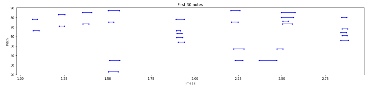
# 查看MIDI文件30个音符的分布情况
plot_piano_roll(raw_notes, count=30)
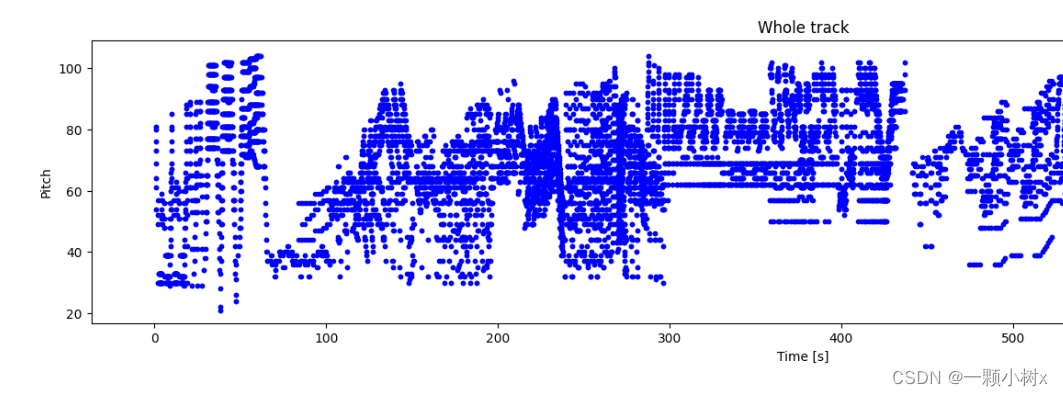
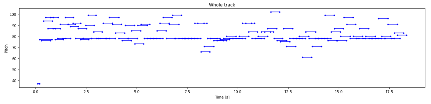
# 绘制整个音轨的音符
plot_piano_roll(raw_notes)查看MIDI文件50个音高和持续时间的情况
绘制整个音轨的音符
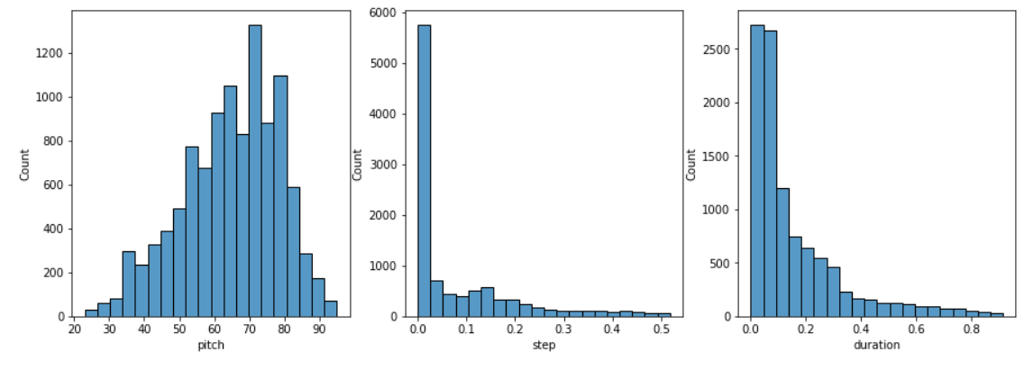
2.4 检查音符分布
检查每个音符变量的分布,通过如下函数实现
def plot_distributions(notes: pd.DataFrame, drop_percentile=2.5):
  plt.figure(figsize=[15, 5])
  plt.subplot(1, 3, 1)
  sns.histplot(notes, x="pitch", bins=20)

  plt.subplot(1, 3, 2)
  max_step = np.percentile(notes['step'], 100 - drop_percentile)
  sns.histplot(notes, x="step", bins=np.linspace(0, max_step, 21))

  plt.subplot(1, 3, 3)
  max_duration = np.percentile(notes['duration'], 100 - drop_percentile)
  sns.histplot(notes, x="duration", bins=np.linspace(0, max_duration, 21))

# 查看音符的分布
plot_distributions(raw_notes)
能看到如下的音符分布:
2.5 创建训练数据集
通过从MIDI文件中提取音符来创建训练数据集,音符用三个变量来表示:pitch(音高)、step(音符名)和 duration(持续时间)。
对于成批的音符序列训练模型;每个样本将包含一系列音符作为输入特征,下一个音符作为标签。通过这种方式,模型将被训练来预测序列中的下一个音符。
以下代码是创建训练数据集的:
key_order = ['pitch', 'step', 'duration']
train_notes = np.stack([all_notes[key] for key in key_order], axis=1)
notes_ds = tf.data.Dataset.from_tensor_slices(train_notes)


# 每个示例将由一系列音符组成作为输入特征,并将下一个音符作为标签。
# 通过这种方式,模型将被训练以预测序列中的下一个音符。
def create_sequences(
    dataset: tf.data.Dataset,
    seq_length: int,
    vocab_size = 128,
) -> tf.data.Dataset:

  seq_length = seq_length+1

  windows = dataset.window(seq_length, shift=1, stride=1,
                              drop_remainder=True)

  flatten = lambda x: x.batch(seq_length, drop_remainder=True)
  sequences = windows.flat_map(flatten)

  def scale_pitch(x):
    x = x/[vocab_size,1.0,1.0]
    return x

  def split_labels(sequences):
    inputs = sequences[:-1]
    labels_dense = sequences[-1]
    labels = {key:labels_dense[i] for i,key in enumerate(key_order)}
    return scale_pitch(inputs), labels

  return sequences.map(split_labels, num_parallel_calls=tf.data.AUTOTUNE)
设置每个示例的序列长度。尝试使用不同的长度(例如,50、100、150),以确定哪种长度最适合数据,或使用超参数调整。词汇表的大小(Vocab_Size)设置为128,表示Pretty_MIDI支持的所有音调。
seq_length = 25
vocab_size = 128
seq_ds = create_sequences(notes_ds, seq_length, vocab_size)
seq_ds.element_spec

batch_size = 64
buffer_size = n_notes - seq_length
train_ds = (seq_ds
            .shuffle(buffer_size)
            .batch(batch_size, drop_remainder=True)
            .cache()
            .prefetch(tf.data.experimental.AUTOTUNE))
三、构建模型
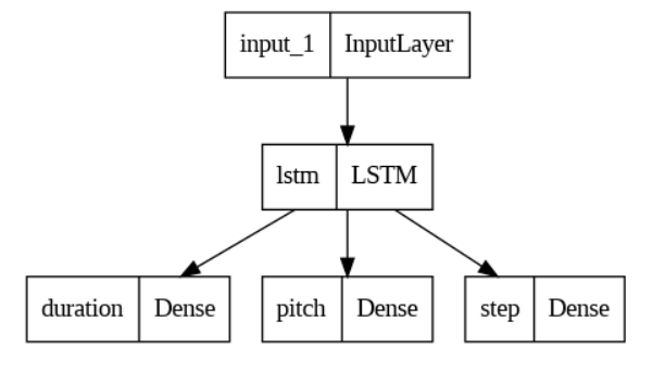
模型输入是序列的音符,输出是一个音符;即:通过输入一段连续的音符,预测下一个音符。
输入:输入的维度是nx3,n是指音符的个数长度,3是指音符使用pitch(音高)、step(音符名)和 duration(持续时间)三个变量来表示;
输出:预测一个音符,设置模型输出的维度是3,表示音符的3个变量。
模型主体:LSTM结构。
损失函数:对于pitch和duration,使用基于均方误差的自定义损失函数。
def mse_with_positive_pressure(y_true: tf.Tensor, y_pred: tf.Tensor):
  mse = (y_true - y_pred) ** 2
  positive_pressure = 10 * tf.maximum(-y_pred, 0.0)
  return tf.reduce_mean(mse + positive_pressure)
下面是搭建网络的代码:
# 设置输入
input_shape = (seq_length, 3)
learning_rate = 0.005

# 模型输入层
inputs = tf.keras.Input(input_shape)

# 使用循环神经网络的变体LSTM层
x = tf.keras.layers.LSTM(128)(inputs)

# 输出层
outputs = {
  'pitch': tf.keras.layers.Dense(128, name='pitch')(x),
  'step': tf.keras.layers.Dense(1, name='step')(x),
  'duration': tf.keras.layers.Dense(1, name='duration')(x),
}

# 构建模型
model = tf.keras.Model(inputs, outputs)

# 定义损失函数
loss = {
      'pitch': tf.keras.losses.SparseCategoricalCrossentropy(
          from_logits=True),
      'step': mse_with_positive_pressure,
      'duration': mse_with_positive_pressure,
}

# 模型训练的优化器
optimizer = tf.keras.optimizers.Adam(learning_rate=learning_rate)

# 编译模型
model.compile(
    loss=loss,
    loss_weights={
        'pitch': 0.05,
        'step': 1.0,
        'duration':1.0,
    },
    optimizer=optimizer,
)

# 设置训练模型时的回调函数
callbacks = [
    tf.keras.callbacks.ModelCheckpoint(
        filepath='./training_checkpoints/ckpt_{epoch}',
        save_weights_only=True),
    tf.keras.callbacks.EarlyStopping(
        monitor='loss',
        patience=5,
        verbose=1,
        restore_best_weights=True),
]
查看一下网络模型:tf.keras.utils.plot_model(model)
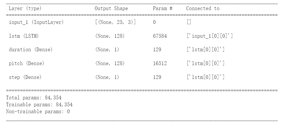
或者用这样方式看看:model.summary()
四、训练模型
这里我们输入准备好的训练集数据,指定训练模型时的回调函数(保存模型权重、自动早停),模型一共训练50轮。
# 模型训练50轮
epochs = 50
# 开始训练模型
history = model.fit(
train_ds,
epochs=epochs,
callbacks=callbacks,
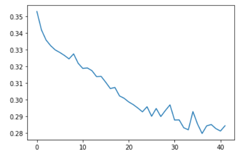
)下图是训练过程的截图,能看到模型训练到42轮时停止了,因为使用EarlyStopping()函数,模型的损失足够小了,就不再训练了。

通常loss越小越好,训练完模型后,画一下损失值的变化过程:
五、使用模型
使用 model.predict( ) 函数,进行预测音符。但要使用模型生成音符,首先需要提供音符的起始序列。
下面的函数,从一系列音符中生成一个音符
def predict_next_note(
    notes: np.ndarray,
    keras_model: tf.keras.Model,
    temperature: float = 1.0) -> int:
  """使用经过训练的序列模型生成标签ID"""

  assert temperature > 0

  # 添加批次维度
  inputs = tf.expand_dims(notes, 0)

  predictions = model.predict(inputs)
  pitch_logits = predictions['pitch']
  step = predictions['step']
  duration = predictions['duration']

  pitch_logits /= temperature
  pitch = tf.random.categorical(pitch_logits, num_samples=1)
  pitch = tf.squeeze(pitch, axis=-1)
  duration = tf.squeeze(duration, axis=-1)
  step = tf.squeeze(step, axis=-1)

  # `step` 和 `duration` 值应该是非负数
  step = tf.maximum(0, step)
  duration = tf.maximum(0, duration)

  return int(pitch), float(step), float(duration)
举一个例子,生成一些音符
temperature = 2.0
num_predictions = 120

sample_notes = np.stack([raw_notes[key] for key in key_order], axis=1)

# 音符的初始序列; 音高被归一化,类似于训练序列
input_notes = (
    sample_notes[:seq_length] / np.array([vocab_size, 1, 1]))

generated_notes = []
prev_start = 0
for _ in range(num_predictions):
  pitch, step, duration = predict_next_note(input_notes, model, temperature)
  start = prev_start + step
  end = start + duration
  input_note = (pitch, step, duration)
  generated_notes.append((*input_note, start, end))
  input_notes = np.delete(input_notes, 0, axis=0)
  input_notes = np.append(input_notes, np.expand_dims(input_note, 0), axis=0)
  prev_start = start

generated_notes = pd.DataFrame(
    generated_notes, columns=(*key_order, 'start', 'end'))
# 查看成的generated_notes前5个音符
generated_notes.head(5)
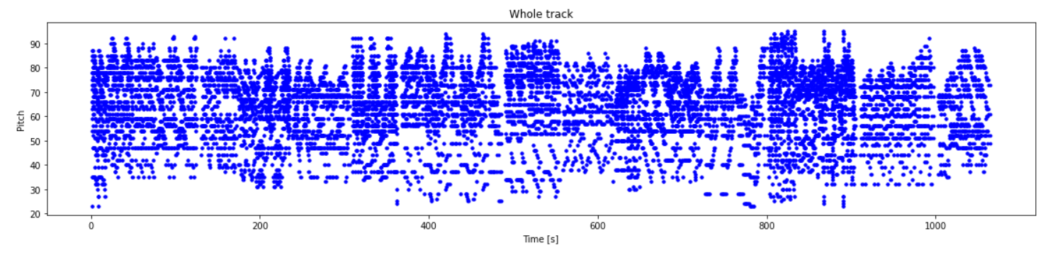
# 查看成的generated_notes的音轨情况
plot_piano_roll(generated_notes)
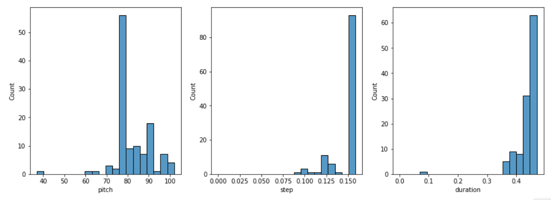
# 查看生成的generated_notes 音符的分布情况
plot_distributions(generated_notes)查看生成的前5个音符,
| pitch | step | duration | start | end | |
|---|---|---|---|---|---|
| 0 | 37 | 0.095633 | 0.092078 | 0.095633 | 0.187710 |
| 1 | 77 | 0.097417 | 0.609462 | 0.193049 | 0.802511 |
| 2 | 76 | 0.089049 | 0.455626 | 0.282099 | 0.737724 |
| 3 | 94 | 0.096575 | 0.443937 | 0.378673 | 0.822611 |
| 4 | 97 | 0.109404 | 0.376604 | 0.488077 | 0.864681 |
查看成的generated_notes的音轨情况
查看生成的generated_notes 音符的分布情况
本文只供大家参考和学习,谢谢~
其它推荐文章:
[1] 【神经网络】综合篇——人工神经网络、卷积神经网络、循环神经网络、生成对抗网络
[2] 手把手搭建一个【卷积神经网络】
[5] 神经网络学习