1. 问题和数据
在本练习中,您将实现神经网络的反向传播算法,并将其应用于手写数字识别任务。(从0到9)。
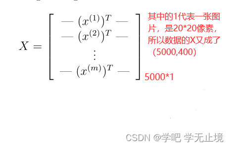
数据集:ex4data1.mat中有5000个训练示例。其中每个训练示例是一个20像素× 20像素的数字灰度图像。每个像素都由一个浮点数表示,该浮点数表示该位置的灰度强度。20 × 20像素网格被“展开”成400维向量。每个训练示例都成为数据矩阵X中的一行。这给了我们一个5000乘400的矩阵X,其中每一行都是一个手写数字图像的训练示例。
因为数据ex2data1.mat太多了,这次就不可能列出来了。但是我们依然可以打印看一下它的特征。
权重集:theta的权重,数据文件是ex4weights.mat
题目已经为我们提供了一组我们训练过的网络参数( Θ 1 Θ_1 Θ1, Θ 2 Θ_2 Θ2)。它们存储在ex4weights.mat中。
在ex4data1.mat的X中,样本分别为手写数字图片0到9,一共10个数字;但是在ex4data1.mat的y中,标签样本总共为1-10,分别用1到9的标签对应表示数字图片到9,用标签10表示数字图片0。
采用One-hot编码,将ex4data1.mat中的y的10种标签用y=的十个不同向量表示,每个向量只有一个1元素,其它元素全为0,依次表示1到10。
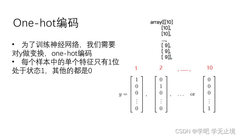
这是为了保证在损失函数中y仍然可以参与运算而设置的。
2. 解决步骤与分析
导入包,numpy和pandas是做运算的库,matplotlib是画图的库。
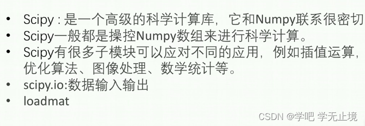
数据集是在MATLAB的格式,所以要加载它在Python,我们需要使用一个SciPy工具。
import numpy as np
import scipy.io as sio
import matplotlib.pyplot as plt
from scipy.optimize import minimize
导入数据集
data = sio.loadmat('ex4data1.mat')
再取出X和y,给X插入一列,打印X的shape出来看一看
```python
raw_X = data['X']
raw_y = data['y']

X = np.insert(raw_X, 0, values=1, axis=1)  # 为了让X能与下面的theta1矩阵相乘,给X插入一列,loc=0,值全是1,这样X的列数就与theta1的行数
# 相同,两矩阵就能做乘法运算了
print('X.shape:', X.shape)
输出结果:
X.shape: (5000, 401)
对y进行独热编码处理:One-hot编码
def one_hot_encoder(raw_y):
    result = []

    for i in raw_y:  # 1到10
        y_temp = np.zeros(10)  # 先设置一个具有10个元素的0列表;np.zeros(数字)表示生成列表;np.zeros(数字,数字)表示生成矩阵
        y_temp[i-1] = 1  # 将索引为i-1的那个元素变为1

        result.append(y_temp)

    return np.array(result)  # 因为上面设置的result是个列表,所以这里还要给它转换成数组格式
调用one_hot_encoder函数,将raw_y转换成One-hot编码后的向量形式,并打印出来看看
y = one_hot_encoder(raw_y)
print('y:', y)
打印输出结果:
y的每一个lable都变成了one-hot的向量形式:
y: [[0. 0. 0. ... 0. 0. 1.]
 [0. 0. 0. ... 0. 0. 1.]
 [0. 0. 0. ... 0. 0. 1.]
 ...
 [0. 0. 0. ... 0. 1. 0.]
 [0. 0. 0. ... 0. 1. 0.]
 [0. 0. 0. ... 0. 1. 0.]]
打印y的shape出来看看:
print('y.shape:', y.shape)
打印输出结果:
y.shape: (5000, 10)
读取权重文件,并将Theta1,Theta2这两列分别赋值
theta = sio.loadmat('ex4weights.mat')
theta1, theta2 = theta['Theta1'], theta['Theta2']
打印theta1, theta2的shape出来看看:
print('theta1.shape:', theta1.shape)
print('theta2.shape:', theta2.shape)
打印输出结果:
theta1.shape: (25, 401)
theta2.shape: (10, 26)
序列化权重参数,并打印序列化处理之后的theta1和2的shape来看看
def serialize(a, b):
    return np.append(a.flatten(), b.flatten())  # 用flatten将a,b都各自拉成一维向量,再用np.append合并成一个一维向量/数组

theta_serialize = serialize(theta1, theta2)
print('theta_serialize:', theta_serialize.shape)  # 得到的一维向量的元素个数=25*401 + 10*26=10285,就是theta1和theta2的所有元素数和
打印输出结果:
theta_serialize: (10285,)
解序列化权重参数,并打印解序列化处理之后的theta1和2的shape来看看
def deserialize(theta_serialize):
    theta1 = theta_serialize[:25*401].reshape(25, 401)  # 将theta_serialize这个一维数组的前25*401个reshape成原来的25*401的样子
    theta2 = theta_serialize[25 * 401:].reshape(10, 26)  # 将theta_serialize这个一维数组的后面的reshape成原来的10*26的样子
    return theta1, theta2
打印输出结果:
theta1.shape: (25, 401)
theta2.shape: (10, 26)
神经网络的原理如下图所示:
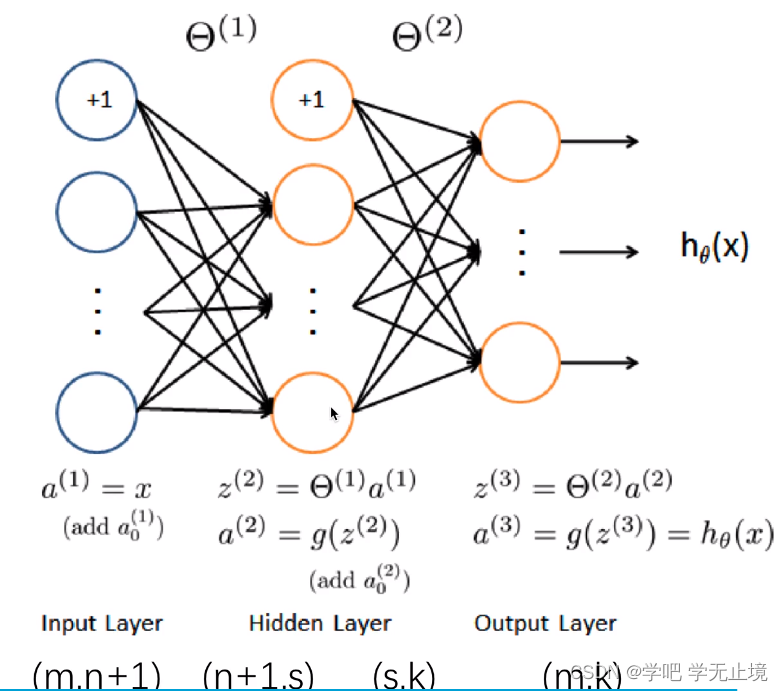
前向传播函数,就相当于cost Fuction,成本代价函数
# sigmoid函数
def sigmoid(z):
    return 1 / (1 + np.exp(-z))

def feed_forward(theta_serialize, X):
    theta1, theta2 = deserialize(theta_serialize)
    a1 = X  # 指定a1

    # 计算z2, a2,并打印a2的shape
    z2 = a1 @ theta.T
    a2 = sigmoid(z2)
    print('a2.shape:', a2.shape)   # a2.shape: (5000, 25)

    # theta2.shape: (10, 26), 为了a2和theta2能做矩阵相乘运算,将a2插入一列,并打印shape来看看
    a2 = np.insert(a2, 0, values=1, axis=1)  # 对a2添加一列全为1的值,(X, 索引=0, 值=0, axis是按行按行插入(0:行、1:列))
    print('a2.shape:', a2.shape)  # a2.shape: (5000, 26)

    # 计算z3, h(其实就是a3,不过是最终值,就叫h了),并打印h的shape
    z3 = a2 @ theta2.T
    h = sigmoid(z3)
    print('h.shape:', h.shape)  # h.shape: (5000, 10)

    return a1, z2, a3, z3, h
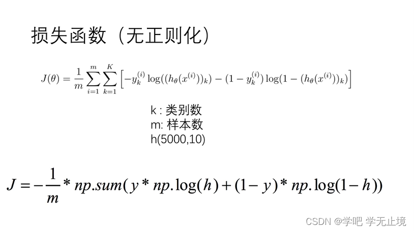
损失函数
损失函数的原理如下图所示:
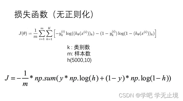
不带正则化的损失函数
def cost(theta_serialize, X, y):
    a1, z2, a2, z3, h = feed_forward(theta_serialize, X)
    J = -np.sum(y*np.log(h)+(1-y)*np.log(1-h)) / len(X)
    return J
调用不带正则化的损失函数,并打印此时的cost来看看
cost(theta_serialize, X, y)
print('cost(theta_serialize, X, y):', cost(theta_serialize, X, y))
打印输出结果:
cost(theta_serialize, X, y): 0.2876291651613189
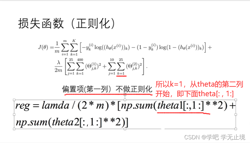
带正则化的损失函数
def reg_cost(theta_serialize, X, y, lamda):
    sum1 = np.sum(np.power(theta1[:, 1], 2))
    sum2 = np.sum(np.power(theta2[:, 1], 2))
    reg = (sum1 + sum2) * lamda / (2*len(X))

    return reg + cost(theta_serialize, X, y)   # 等于不带正则化的+带带正则化的
设置lamda=1时,调用不带正则化的损失函数,并打印此时的cost来看看
lamda = 1
reg_cost(theta_serialize, X, y, lamda)
print('reg_cost(theta_serialize, X, y, lamda):', reg_cost(theta_serialize, X, y, lamda))
打印输出结果:
reg_cost(theta_serialize, X, y, lamda): 0.2890868603763652
带正则化的损失函数
def reg_cost(theta_serialize, X, y, lamda):
    sum1 = np.sum(np.power(theta1[:, 1], 2))
    sum2 = np.sum(np.power(theta2[:, 1], 2))
    reg = (sum1 + sum2) * lamda / (2*len(X))

    return reg + cost(theta_serialize, X, y)  # 等于不带正则化的+带带正则化的

lamda = 1
reg_cost(theta_serialize, X, y, lamda)
print('reg_cost(theta_serialize, X, y, lamda):', reg_cost(theta_serialize, X, y, lamda))
打印输出结果:
reg_cost(theta_serialize, X, y, lamda): 0.28897007621372756
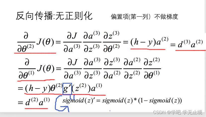
反向传播函数, 就相当于梯度下降函数
def sigmoid_gradient(z):
    return sigmoid(z) * (1-sigmoid(z))

# 不带正则化的梯度
def gradient(theta_serialize, X, y):
    theta1, theta2 = deserialize(theta_serialize)
    a1, z2, a2, z3, h = feed_forward(theta_serialize, X)
    d3 = h - y
    d2 = d3 @ theta2[:, 1:] * sigmoid_gradient(z2)
    D2 = (d3.T @ a2) / len(X)
    D1 = (d2.T @ a1) / len(X)

    return serialize(D1, D2)  # 返回D1和D2,并序列化一下
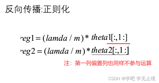
带正则化的梯度
def reg_gradient(theta_serialize, X, y, lamda):
    D = gradient(theta_serialize, X, y)  # 就是在获取不带正则化的梯度的结果的情况下
    D1, D2 = deserialize(D)  # 将结果D1, D2先解序列化

    theta1, theta2 = deserialize(theta_serialize)
    D1[:, 1:] = D1[:, 1:] + theta1[:, 1:] * lamda / len(X)  # 在原来的D1基础上加上theta1的正则化部分
    D2[:, 1:] = D2[:, 1:] + theta2[:, 1:] * lamda / len(X)  # 在原来的D2基础上加上theta2的正则化部分

    return serialize(D1, D2)  # 返回新的D1和D2,并序列化一下
神经网络的优化
用scipy进行优化
不加正则化,正确率为0.9998,显然过拟合
def nn_training(X, y):
    init_theta = np.random.uniform(-0.5, 0.5, 10285)  # 取初始的theta值,取值范围从0.5到0.5,取10285个
    res = minimize(fun=cost,  # 要优化的函数
                   x0=init_theta,  # 参数初始值,init_theta一开始是零数组
                   args=(X, y),   # ??不太懂,网上查一下
                   method='TNC',  # 选择‘TNC’的优化方法,好像是牛顿迭代法,具体原理不用管
                   jac=gradient,  # 梯度向量
                   options={

    'maxiter': 300})  # 设置最大迭代次数为300次

    return res

res = nn_training(X, y)  # 调用神经网络优化函数,scipy库自动进行优化
raw_y = data['y'].reshape(5000,)  # 将原本数据集中y标签raw_y取出,并reshape成一维向量,便于下面比较并计算准确度

_,_,_,_,h = feed_forward(res.x, X)  # _,_,_,_,h是省略写法,其实就是feed_forward()函数最后return的 a1, z2, a2, z3, h,将优化过的
# 结果中res的x列和原本的数据集X带入前向传播函数,把feed_forward()函数计算后结果分别传值给a1, z2, a2, z3, h
y_pred = np.argmax(h, axis=1) + 1  # arg是np中的比较函数,max是选大的意思;axis=0是行,axis=1就是将对同一行的每一列去比较,哪一个比较
    # 大我们就将它的索引返回回来,比如第一个位置的结果最大,就返回它的索引,但结果是0,所以要对返回的索引加1
acc = np.mean(y_pred == raw_y)  # 计算准确率accuracy; 求预测值y_pred等于真实值raw_y的个数,再求平均值
print('acc:', acc)
打印输出结果:
acc: 0.9972
加入正则化,正确率降低,一定程度上解决了过拟合
def reg_nn_training(X, y, lamda):
    init_theta = np.random.uniform(-0.5, 0.5, 10285)
    res = minimize(fun=reg_cost,
                   x0=init_theta,
                   args=(X, y, lamda),
                   method='TNC',
                   jac=reg_gradient,
                   options={

    'maxiter': 300})
    return res


lamda = 10
res = reg_nn_training(X, y, lamda)
_,_,_,_,h = feed_forward(res.x, X)
y_predict = np.argmax(h, axis=1) + 1
acc = np.mean(y_predict == raw_y)
print('acc:', acc)  # 加上正则化这步,正确率为0.9384,正常了许多
打印输出结果:
acc: 0.9384
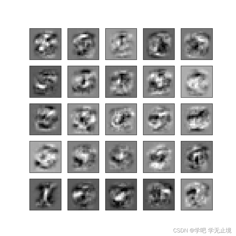
可视化隐藏层特征向量
def plot_hidden_layer(theta):
    theta1,_ = deserialize(theta)  # theta1,_为省略写法,其实就是theta1,theta2
    hidden_layer = theta1[:, 1:]  # 其实就是25,400; 400是图片像素20*20,所以其实可以理解为25张像素为20*20的图片
    print('hidden_layer.shape:', hidden_layer.shape)

    fig, ax = plt.subplots(ncols=5, nrows=5, figsize=(8, 8), sharex=True, sharey=True)  # ncols为5列, nrows=5行;画布大
    # 小8*8;共享x轴的刻度,共享y轴的刻度(原来是每个小格有一套x轴和y轴,现在是整体只有一个x轴和y轴

    for r in range(5):
        for c in range(5):

            ax[r, c].imshow(hidden_layer[5 * r + c].reshape(20, 20).T, cmap='gray_r')   # 将hidden_layer由400reshape成20*20的格式,才是图片,再.T转置才是我们
            # 能看懂的图片; cmap='gray_r'是设置颜色

    plt.xticks([])  # 然后再去掉横坐标值
    plt.yticks([])  # 然后再去掉纵坐标值
    plt.show()

plot_hidden_layer(res.x)
打印输出结果:
hidden_layer.shape: (25, 400)
3. 源代码
# -*- coding: utf-8 -*-
"""
Created on Sat June 11 10:14:26 2022
@author: wzj
python version: python 3.9

Title: 利用神经网络的反向传播算法( backpropagation algorithm for neural networks),并将其应用于手写数字识别。

数据集:数据文件是ex4data1.mat
权重集:theta的权重,数据文件是ex4weights.mat
"""

import numpy as np
import scipy.io as sio
import matplotlib.pyplot as plt
from scipy.optimize import minimize

data = sio.loadmat('ex4data1.mat')
raw_X = data['X']
raw_y = data['y']

X = np.insert(raw_X, 0, values=1, axis=1)  # 为了让X能与下面的theta1矩阵相乘,给X插入一列,loc=0,值全是1,这样X的列数就与theta1的行数
# 相同,两矩阵就能做乘法运算了
print('X.shape:', X.shape)
# ---------------------------

test = np.zeros(10)
print('test:', test)
# ---------------------------
# 对y进行独热编码处理:One-hot编码
def one_hot_encoder(raw_y):
    result = []

    for i in raw_y:  # 1到10
        y_temp = np.zeros(10)  # 先设置一个具有10个元素的0列表;np.zeros(数字)表示生成列表;np.zeros(数字,数字)表示生成矩阵
        y_temp[i-1] = 1  # 将索引为i-1的那个元素变为1

        result.append(y_temp)

    return np.array(result)  # 因为上面设置的result是个列表,所以这里还要给它转换成数组格式
# ---------------------------
y = one_hot_encoder(raw_y)
print('y:', y)
print('y.shape:', y.shape)
# ---------------------------

# ---------------------------
# 读取权重文件,并将Theta1,Theta2这两列分别赋值
theta = sio.loadmat('ex4weights.mat')
theta1, theta2 = theta['Theta1'], theta['Theta2']
print('theta1.shape:', theta1.shape)
print('theta2.shape:', theta2.shape)
# ---------------------------

# ---------------------------
# 序列化权重参数
def serialize(a, b):
    return np.append(a.flatten(), b.flatten())  # 用flatten将a,b都各自拉成一维向量,再用np.append合并成一个一维向量/数组

theta_serialize = serialize(theta1, theta2)
print('theta_serialize:', theta_serialize.shape)  # 得到的一维向量的元素个数=25*401 + 10*26=10285,就是theta1和theta2的所有元素数和
# ---------------------------

# ---------------------------
# 解序列化权重参数
def deserialize(theta_serialize):
    theta1 = theta_serialize[:25*401].reshape(25, 401)  # 将theta_serialize这个一维数组的前25*401个reshape成原来的25*401的样子
    theta2 = theta_serialize[25 * 401:].reshape(10, 26)  # 将theta_serialize这个一维数组的后面的reshape成原来的10*26的样子
    return theta1, theta2

theta1, theta2 = deserialize(theta_serialize)
print('theta1.shape:', theta1.shape)  # 检查解序列化权重参数后theta1和2的shape
print('theta2.shape:', theta2.shape)
# ---------------------------

# ---------------------------
# 前向传播函数,就相当于cost Fuction,成本代价函数
# sigmoid函数
def sigmoid(z):
    return 1 / (1 + np.exp(-z))

def feed_forward(theta_serialize, X):
    theta1, theta2 = deserialize(theta_serialize)
    a1 = X  # 指定a1

    # 计算z2, a2,并打印a2的shape
    z2 = a1 @ theta1.T
    a2 = sigmoid(z2)
    # print('a2.shape:', a2.shape)   # a2.shape: (5000, 25)

    # theta2.shape: (10, 26), 为了a2和theta2能做矩阵相乘运算,将a2插入一列,并打印shape来看看
    a2 = np.insert(a2, 0, values=1, axis=1)  # 对a2添加一列全为1的值,(X, 索引=0, 值=0, axis是按行按行插入(0:行、1:列))
    # print('a2.shape:', a2.shape)  # a2.shape: (5000, 26)

    # 计算z3, h(其实就是a3,不过是最终值,就叫h了),并打印h的shape
    z3 = a2 @ theta2.T
    h = sigmoid(z3)
    # print('h.shape:', h.shape)  # h.shape: (5000, 10)

    return a1, z2, a2, z3, h
# ---------------------------

# ---------------------------
# 损失函数
# 不带正则化的损失函数
def cost(theta_serialize, X, y):
    a1, z2, a2, z3, h = feed_forward(theta_serialize, X)
    J = -np.sum(y*np.log(h + 1e-5)+(1-y)*np.log(1-h + 1e-5)) / len(X)
    return J

cost(theta_serialize, X, y)
print('cost(theta_serialize, X, y):', cost(theta_serialize, X, y))


# 带正则化的损失函数
def reg_cost(theta_serialize, X, y, lamda):
    sum1 = np.sum(np.power(theta1[:, 1], 2))
    sum2 = np.sum(np.power(theta2[:, 1], 2))
    reg = (sum1 + sum2) * lamda / (2*len(X))

    return reg + cost(theta_serialize, X, y)  # 等于不带正则化的+带带正则化的

lamda = 1
reg_cost(theta_serialize, X, y, lamda)
print('reg_cost(theta_serialize, X, y, lamda):', reg_cost(theta_serialize, X, y, lamda))
# ---------------------------

# ---------------------------
# 反向传播函数, 就相当于梯度下降函数
def sigmoid_gradient(z):
    return sigmoid(z) * (1-sigmoid(z))

# 不带正则化的梯度
def gradient(theta_serialize, X, y):
    theta1, theta2 = deserialize(theta_serialize)
    a1, z2, a2, z3, h = feed_forward(theta_serialize, X)
    d3 = h - y
    d2 = d3 @ theta2[:, 1:] * sigmoid_gradient(z2)
    D2 = (d3.T @ a2) / len(X)
    D1 = (d2.T @ a1) / len(X)

    return serialize(D1, D2)  # 返回D1和D2,并序列化一下

# 带正则化的梯度
def reg_gradient(theta_serialize, X, y, lamda):
    D = gradient(theta_serialize, X, y)  # 就是在获取不带正则化的梯度的结果的情况下
    D1, D2 = deserialize(D)  # 将结果D1, D2先解序列化

    theta1, theta2 = deserialize(theta_serialize)
    D1[:, 1:] = D1[:, 1:] + theta1[:, 1:] * lamda / len(X)  # 在原来的D1基础上加上theta1的正则化部分
    D2[:, 1:] = D2[:, 1:] + theta2[:, 1:] * lamda / len(X)  # 在原来的D2基础上加上theta2的正则化部分

    return serialize(D1, D2)  # 返回新的D1和D2,并序列化一下
# ---------------------------

# ---------------------------
# 神经网络的优化
# 用scipy进行优化
# 不加正则化,正确率为0.9998,显然过拟合
def nn_training(X, y):
    init_theta = np.random.uniform(-0.5, 0.5, 10285)  # 取初始的theta值,取值范围从0.5到0.5,取10285个
    res = minimize(fun=cost,  # 要优化的函数
                   x0=init_theta,  # 参数初始值,init_theta一开始是零数组
                   args=(X, y),   # ??不太懂,网上查一下
                   method='TNC',  # 选择‘TNC’的优化方法,好像是牛顿迭代法,具体原理不用管
                   jac=gradient,  # 梯度向量
                   options={

    'maxiter': 300})  # 设置最大迭代次数为300次

    return res

res = nn_training(X, y)  # 调用神经网络优化函数,scipy库自动进行优化
raw_y = data['y'].reshape(5000,)  # 将原本数据集中y标签raw_y取出,并reshape成一维向量,便于下面比较并计算准确度

_,_,_,_,h = feed_forward(res.x, X)  # _,_,_,_,h是省略写法,其实就是feed_forward()函数最后return的 a1, z2, a2, z3, h,将优化过的
# 结果中res的x列和原本的数据集X带入前向传播函数,把feed_forward()函数计算后结果分别传值给a1, z2, a2, z3, h
y_pred = np.argmax(h, axis=1) + 1  # arg是np中的比较函数,max是选大的意思;axis=0是行,axis=1就是将对同一行的每一列去比较,哪一个比较
    # 大我们就将它的索引返回回来,比如第一个位置的结果最大,就返回它的索引,但结果是0,所以要对返回的索引加1
acc = np.mean(y_pred == raw_y)  # 计算准确率accuracy; 求预测值y_pred等于真实值raw_y的个数,再求平均值
print('acc:', acc)

# ---------------------------
# 加入正则化,正确率降低,一定程度上解决了过拟合
def reg_nn_training(X, y, lamda):
    init_theta = np.random.uniform(-0.5, 0.5, 10285)
    res = minimize(fun=reg_cost,
                   x0=init_theta,
                   args=(X, y, lamda),
                   method='TNC',
                   jac=reg_gradient,
                   options={

    'maxiter': 300})
    return res


lamda = 10
res = reg_nn_training(X, y, lamda)
_,_,_,_,h = feed_forward(res.x, X)
y_predict = np.argmax(h, axis=1) + 1
acc = np.mean(y_predict == raw_y)
print('acc:', acc)  # 加上正则化这步,正确率为0.9384,正常了许多
# ---------------------------

# ---------------------------
# 可视化隐藏层特征向量
def plot_hidden_layer(theta):
    theta1,_ = deserialize(theta)  # theta1,_为省略写法,其实就是theta1,theta2
    hidden_layer = theta1[:, 1:]  # 其实就是25,400; 400是图片像素20*20,所以其实可以理解为25张像素为20*20的图片
    print('hidden_layer.shape:', hidden_layer.shape)

    fig, ax = plt.subplots(ncols=5, nrows=5, figsize=(8, 8), sharex=True, sharey=True)  # ncols为5列, nrows=5行;画布大
    # 小8*8;共享x轴的刻度,共享y轴的刻度(原来是每个小格有一套x轴和y轴,现在是整体只有一个x轴和y轴

    for r in range(5):
        for c in range(5):

            ax[r, c].imshow(hidden_layer[5 * r + c].reshape(20, 20).T, cmap='gray_r')   # 将hidden_layer由400reshape成20*20的格式,才是图片,再.T转置才是我们
            # 能看懂的图片; cmap='gray_r'是设置颜色

    plt.xticks([])  # 然后再去掉横坐标值
    plt.yticks([])  # 然后再去掉纵坐标值
    plt.show()

plot_hidden_layer(res.x)
参考文献:
[1] https://www.bilibili.com/video/BV1W4411o7gG?p=8&spm_id_from=pageDriver&vd_source=72e4369cf6b54497a1e04f2071a47a1e
[2] https://github.com/PlayPurEo/ML-and-DL/blob/master/basic-model/4.back%20propagation/bp.py