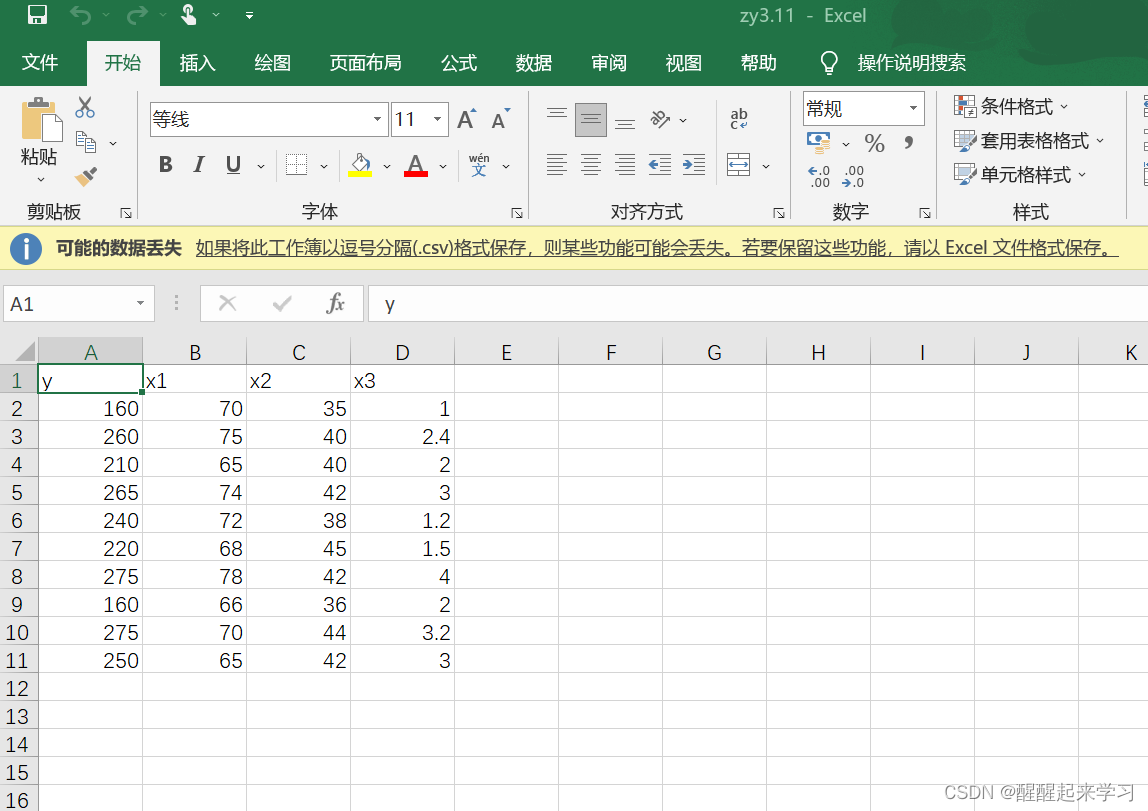
研究货运总量 y (万吨)与工业总产值 x1(亿元)、农业总产值 x2(亿元),居民非商品支出 X3 (亿元)的关系。数据见表3-9。
(1)计算出 y , x1 ,x2, x3 的相关系数矩阵。
(2)求 y 关于 x1 ,x2, x3 的三元线性回归方程。
(3)对所求得的方程做拟合优度检验。
(4)对回归方程做显著性检验。
(5)对每一个回归系数做显著性检验。
(6)如果有的回归系数没通过显著性检验,将其剔除,重新建立回归方程归方程的显著性检验和回归系数的显著性检验。
(7)求出每一个回归系数的置信水平为95%的置信区间
8)求标准化回归方程。
(9)求当X01=75,X02=42,X03=3.1时的,给定置信水平为95%,用算精确置信区间,手工计算近似预测区间
(10)结合回归方程对问题做一些基本分析
表3-9
注:每一小问的运行结果我以备注的形式 放在代码段里面
#导入需要的库和数据
import numpy as np
import statsmodels.api as sm
import statsmodels.formula.api as smf
from statsmodels.stats.api import anova_lm
import matplotlib.pyplot as plt
import pandas as pd
from patsy import dmatrices

# Load data
df = pd.read_csv('C:\\Users\\joyyiyi\\Desktop\\zy3.11.csv',encoding='gbk')
#解决第(!)问
#计算相关系数
cor_matrix = df.corr(method='pearson')  # 使用皮尔逊系数计算列与列的相关性
# cor_matrix = df.corr(method='kendall')
# cor_matrix = df.corr(method='spearman')

print(cor_matrix)

'''
结果:
C:\Users\joyyiyi\AppData\Local\Programs\Python\Python39\python.exe C:/Users/joyyiyi/PycharmProjects/pythonProject6/0.py
           y        x1        x2        x3
y   1.000000  0.555653  0.730620  0.723535
x1  0.555653  1.000000  0.112951  0.398387
x2  0.730620  0.112951  1.000000  0.547474
x3  0.723535  0.398387  0.547474  1.000000

Process finished with exit code 0
'''
#解决第(2)(3)(4)(5)问
result = smf.ols('y~x1+x2+x3',data=df).fit()
#print(result.params) #输出回归系数
print(result.summary())
print("\n")
print(result.pvalues) #输出p值
#
'''
运行结果:
C:\Users\joyyiyi\AppData\Local\Programs\Python\Python39\python.exe C:/Users/joyyiyi/PycharmProjects/pythonProject6/0.py
OLS Regression Results
==============================================================================
Dep. Variable: y R-squared: 0.806
Model: OLS Adj. R-squared: 0.708
Method: Least Squares F-statistic: 8.283
Date: Wed, 09 Nov 2022 Prob (F-statistic): 0.0149
Time: 11:15:30 Log-Likelihood: -43.180
No. Observations: 10 AIC: 94.36
Df Residuals: 6 BIC: 95.57
Df Model: 3
Covariance Type: nonrobust
==============================================================================
coef std err t P>|t| [0.025 0.975]
------------------------------------------------------------------------------
Intercept -348.2802 176.459 -1.974 0.096 -780.060 83.500
x1 3.7540 1.933 1.942 0.100 -0.977 8.485
x2 7.1007 2.880 2.465 0.049 0.053 14.149
x3 12.4475 10.569 1.178 0.284 -13.415 38.310
==============================================================================
Omnibus: 0.619 Durbin-Watson: 1.935
Prob(Omnibus): 0.734 Jarque-Bera (JB): 0.562
Skew: 0.216 Prob(JB): 0.755
Kurtosis: 1.922 Cond. No. 1.93e+03
==============================================================================
Notes:
[1] Standard Errors assume that the covariance matrix of the errors is correctly specified.
[2] The condition number is large, 1.93e+03. This might indicate that there are
strong multicollinearity or other numerical problems.
Intercept 0.095855
x1 0.100197
x2 0.048769
x3 0.283510
dtype: float64
Process finished with exit code 0
'''
'''
(2)回答:线性方程:
Y=-348.2802+3.7540x1+7.1007x2+12.4475x3
(3)回答:R方=0.806,调整后R方=0.708
#或者说R=0.806>R0.05(8)=0.632,所以接受原假设,说明x与y有显著的线性关系
#或者说调整后的决定系数为0.708,说明回归方程对样本观测值的拟合程度较好。
(4)回答:做(F检验)
#原假设H0=β1=β2=β3=0
# F=8.283>F0.05(3,6)=4.76,或者说P=0.0149<α=0.05,说明拒绝原假设H0,x与y有显著的线性关系
(5)x1,x2,x3的t值分别为:
t1=1.942<t0.05(8)=1.943或者α=0.100>α=0.05,所以接受原假设,说明x1对y没有显著的影响
t2=2.465>t0.05(8)=1.943或者α=0.049<α=0.05,所以拒绝原假设,说明x1对y有显著的影响
t3=1.178<t0.05(8)=1.943或者α=0.284>α=0.05,所以接受原假设,说明x1对y没有显著的影响
'''
#在第(5)中发现除了x2外其他回归系数都未通过显著性检验,首先剔除x3看看效果
result = smf.ols('y~x1+x2',data=df).fit()

#print(result.params)    #输出回归系数
print(result.summary())
print("\n")
print(result.pvalues)     #输出p值

'''
运行结果:
C:\Users\joyyiyi\AppData\Local\Programs\Python\Python39\python.exe C:/Users/joyyiyi/PycharmProjects/pythonProject6/0.py
                            OLS Regression Results
==============================================================================
Dep. Variable:                      y   R-squared:                       0.761
Model:                            OLS   Adj. R-squared:                  0.692
Method:                 Least Squares   F-statistic:                     11.12
Date:                Wed, 09 Nov 2022   Prob (F-statistic):            0.00672
Time:                        11:49:08   Log-Likelihood:                -44.220
No. Observations:                  10   AIC:                             94.44
Df Residuals:                       7   BIC:                             95.35
Df Model:                           2
Covariance Type:            nonrobust
==============================================================================
                 coef    std err          t      P>|t|      [0.025      0.975]
------------------------------------------------------------------------------
Intercept   -459.6237    153.058     -3.003      0.020    -821.547     -97.700
x1             4.6756      1.816      2.575      0.037       0.381       8.970
x2             8.9710      2.468      3.634      0.008       3.134      14.808
==============================================================================
Omnibus:                        1.265   Durbin-Watson:                   1.895
Prob(Omnibus):                  0.531   Jarque-Bera (JB):                0.631
Skew:                          -0.587   Prob(JB):                        0.730
Kurtosis:                       2.630   Cond. No.                     1.63e+03
==============================================================================

Notes:
[1] Standard Errors assume that the covariance matrix of the errors is correctly specified.
[2] The condition number is large, 1.63e+03. This might indicate that there are
strong multicollinearity or other numerical problems.


Intercept    0.019859
x1           0.036761
x2           0.008351
dtype: float64

Process finished with exit code 0

'''

#第(6)问回答:
在剔除x3后,回归方程Y=-459.6237+4.6756x1+8.9710x2
的拟合优度R2=0.761,F值=11.12(有所提高),回归系数的P值均小于0.05 因此回归系数均通过显著性t检验

#第(7)问回答:
通过summary()输出的回归结果最右边“[0.025      0.975]”这个位置可以看到
常数项,x1,x2的回归系数置信水平为95%的置信区间分别为:[-821.547,-97.700],[0.381,8.970],[3.134,14.808]
#标准化
dfnorm = (df-df.mean())/df.std()
new = pd.Series({'x1': 4000,'x2': 3300,'x3': 113000,'x4': 50.0,'x5': 1000.0})
newnorm = (new-df.mean())/df.std()
#标准化后构建无截距模型
resultnorm = smf.ols('y~x1+x2',data=dfnorm).fit()

print(resultnorm.summary())
'''
运行结果:
                            OLS Regression Results
==============================================================================
Dep. Variable:                      y   R-squared:                       0.761
Model:                            OLS   Adj. R-squared:                  0.692
Method:                 Least Squares   F-statistic:                     11.12
Date:                Fri, 11 Nov 2022   Prob (F-statistic):            0.00672
Time:                        22:51:34   Log-Likelihood:                -6.5156
No. Observations:                  10   AIC:                             19.03
Df Residuals:                       7   BIC:                             19.94
Df Model:                           2
Covariance Type:            nonrobust
==============================================================================
                 coef    std err          t      P>|t|      [0.025      0.975]
------------------------------------------------------------------------------
Intercept  -8.327e-17      0.175  -4.75e-16      1.000      -0.415       0.415
x1             0.4792      0.186      2.575      0.037       0.039       0.919
x2             0.6765      0.186      3.634      0.008       0.236       1.117
==============================================================================
Omnibus:                        1.265   Durbin-Watson:                   1.895
Prob(Omnibus):                  0.531   Jarque-Bera (JB):                0.631
Skew:                          -0.587   Prob(JB):                        0.730
Kurtosis:                       2.630   Cond. No.                         1.12
==============================================================================

Notes:
[1] Standard Errors assume that the covariance matrix of the errors is correctly specified.

Process finished with exit code 0

'''
第(8)问:
标准化后的回归方程为:
y=0.4792x1+0.6765x2-8.327e-17
# Load data
df = pd.read_csv('C:\\Users\\joyyiyi\\Desktop\\zy3.11.csv',encoding='gbk')
# print(df)
result = smf.ols('y~x1+x2',data=df).fit()
#标准化
dfnorm = (df-df.mean())/df.std()
new = pd.Series({'x1': 75,'x2': 42})
newnorm = (new-df.mean())/df.std()
#标准化后构建无截距模型
resultnorm = smf.ols('y~x1+x2',data=dfnorm).fit()
#单值预测
predictnorm = resultnorm.predict(pd.DataFrame({'x1': [newnorm['x1']],'x2': [newnorm['x2']]}))
#因为单值预测是基于标准化后的模型,需要对y值还原,y值还原方法:
ypredict = predictnorm*df.std()['y'] + df.mean()['y']
print("ypredict:")
print(ypredict)
#区间
predictions = result.get_prediction(pd.DataFrame({'x1': [75],'x2': [42]}))
print('置信水平为95%,区间预测:')
print(predictions.summary_frame(alpha=0.05))
#近似预测区间:
ylow=267.83-2*np.sqrt(result.scale)
yup=267.83+2*np.sqrt(result.scale)
print(ylow,yup)
'''
运行结果:
C:\Users\joyyiyi\AppData\Local\Programs\Python\Python39\python.exe C:/Users/joyyiyi/PycharmProjects/pythonProject6/回归作业.py
ypredict:
0 267.829001
dtype: float64
置信水平为95%,区间预测:
mean mean_se ... obs_ci_lower obs_ci_upper
0 267.829001 11.782559 ... 204.435509 331.222493
[1 rows x 6 columns]
219.66776823691464 315.99223176308533
Process finished with exit code 0
'''
第(9)问:
y0的预测值为267.829;
y0预测值的置信水平为95%的精确置信区间为:[204.44,331.22],
y0近似预测区间为:[219.67,315.99]
在做这次作业的时候因为不确定答案对不对,参考了csdn的另一位朋友的文章:
R语言之多元线性回归xt3.11_princess yang的博客-CSDN博客_为了研究货运量y与工业总产值x1
这篇写的很好,比我更有条理哦