文章目录
1、Curve Fitting
到目前为止,我们看到的示例都是没有数据的简单优化问题。最小二乘和非线性最小二乘分析的原始目的是对数据进行曲线拟合。
以一个简单的曲线拟合的问题为例。采样点是根据曲线 y = e 0.3 x + 0.1 y = e^{0.3x + 0.1} y=e0.3x+0.1 生成,并且添加标准差 σ = 0.2 σ=0.2 σ=0.2 的高斯噪声。我们用下列带未知参数的方程来拟合这些采样点: y = e m x + c . y = e^{mx + c}. y=emx+c.
1.1、残差定义
首先定义一个模板对象来计算残差。每一个观察值(采样点)都有一个残差,
struct ExponentialResidual {


  ExponentialResidual(double x, double y)
      : x_(x), y_(y) {

    }

  template <typename T>
  bool operator()(const T* const m, const T* const c, T* residual) const {


    residual[0] = y_ - exp(m[0] * x_ + c[0]);
    return true;
  }

 private:
  // Observations for a sample.
  const double x_;
  const double y_;
};
1.2、 Problem问题构造
假设观测数据是一个名为data的2n大小的的数组,为每一个观察值创建一个CostFunction的问题(problem)构造是一个简单的事。
double m = 0.0;
double c = 0.0;

Problem problem;
for (int i = 0; i < kNumObservations; ++i) {


  CostFunction* cost_function =
       new AutoDiffCostFunction<ExponentialResidual, 1, 1, 1>(
           new ExponentialResidual(data[2 * i], data[2 * i + 1]));
  problem.AddResidualBlock(cost_function, nullptr, &m, &c);
}
*/
与Hello World的f(x)=10−x对比:
struct CostFunctor {


   template <typename T>
   bool operator()(const T* const x, T* residual) const {


     residual[0] = T(10.0) - x[0];
     return true;
   }
};
CostFunction* cost_function =
     new AutoDiffCostFunction<CostFunctor, 1, 1>(new CostFunctor);
problem.AddResidualBlock(cost_function, NULL, &x);
对比结果:
- 1.在Hello World中,CostFunctor中是没有(显式)构造函数的,也就同样没有了初始值。所以在构造对象时,可以直接New CostFunctor。而在本节的例子中,构造对象时还要加上初始值,即
new ExponentialResidual(data[2 * i], data[2 * i + 1])); - 2.在AutoDiffCostFunction的模板中,本例中一共有三个1,而在Hello World中,只有两个1,即residual和x的维度。注意先是残差,后是输入参数,而且一一对应。
1.3、完整代码
// Ceres Solver - A fast non-linear least squares minimizer
// Copyright 2015 Google Inc. All rights reserved.
// http://ceres-solver.org/
//
// Redistribution and use in source and binary forms, with or without
// modification, are permitted provided that the following conditions are met:
//
// * Redistributions of source code must retain the above copyright notice,
//   this list of conditions and the following disclaimer.
// * Redistributions in binary form must reproduce the above copyright notice,
//   this list of conditions and the following disclaimer in the documentation
//   and/or other materials provided with the distribution.
// * Neither the name of Google Inc. nor the names of its contributors may be
//   used to endorse or promote products derived from this software without
//   specific prior written permission.
//
// THIS SOFTWARE IS PROVIDED BY THE COPYRIGHT HOLDERS AND CONTRIBUTORS "AS IS"
// AND ANY EXPRESS OR IMPLIED WARRANTIES, INCLUDING, BUT NOT LIMITED TO, THE
// IMPLIED WARRANTIES OF MERCHANTABILITY AND FITNESS FOR A PARTICULAR PURPOSE
// ARE DISCLAIMED. IN NO EVENT SHALL THE COPYRIGHT OWNER OR CONTRIBUTORS BE
// LIABLE FOR ANY DIRECT, INDIRECT, INCIDENTAL, SPECIAL, EXEMPLARY, OR
// CONSEQUENTIAL DAMAGES (INCLUDING, BUT NOT LIMITED TO, PROCUREMENT OF
// SUBSTITUTE GOODS OR SERVICES; LOSS OF USE, DATA, OR PROFITS; OR BUSINESS
// INTERRUPTION) HOWEVER CAUSED AND ON ANY THEORY OF LIABILITY, WHETHER IN
// CONTRACT, STRICT LIABILITY, OR TORT (INCLUDING NEGLIGENCE OR OTHERWISE)
// ARISING IN ANY WAY OUT OF THE USE OF THIS SOFTWARE, EVEN IF ADVISED OF THE
// POSSIBILITY OF SUCH DAMAGE.
//
// Author: [email protected] (Sameer Agarwal)

#include "ceres/ceres.h"
#include "glog/logging.h"

using ceres::AutoDiffCostFunction;
using ceres::CostFunction;
using ceres::Problem;
using ceres::Solver;
using ceres::Solve;

// Data generated using the following octave code.
//   randn('seed', 23497);
//   m = 0.3;
//   c = 0.1;
//   x=[0:0.075:5];
//   y = exp(m * x + c);
//   noise = randn(size(x)) * 0.2;
//   y_observed = y + noise;
//   data = [x', y_observed'];

const int kNumObservations = 67;
const double data[] = {


  0.000000e+00, 1.133898e+00,
  7.500000e-02, 1.334902e+00,
  1.500000e-01, 1.213546e+00,
  2.250000e-01, 1.252016e+00,
  3.000000e-01, 1.392265e+00,
  3.750000e-01, 1.314458e+00,
  4.500000e-01, 1.472541e+00,
  5.250000e-01, 1.536218e+00,
  6.000000e-01, 1.355679e+00,
  6.750000e-01, 1.463566e+00,
  7.500000e-01, 1.490201e+00,
  8.250000e-01, 1.658699e+00,
  9.000000e-01, 1.067574e+00,
  9.750000e-01, 1.464629e+00,
  1.050000e+00, 1.402653e+00,
  1.125000e+00, 1.713141e+00,
  1.200000e+00, 1.527021e+00,
  1.275000e+00, 1.702632e+00,
  1.350000e+00, 1.423899e+00,
  1.425000e+00, 1.543078e+00,
  1.500000e+00, 1.664015e+00,
  1.575000e+00, 1.732484e+00,
  1.650000e+00, 1.543296e+00,
  1.725000e+00, 1.959523e+00,
  1.800000e+00, 1.685132e+00,
  1.875000e+00, 1.951791e+00,
  1.950000e+00, 2.095346e+00,
  2.025000e+00, 2.361460e+00,
  2.100000e+00, 2.169119e+00,
  2.175000e+00, 2.061745e+00,
  2.250000e+00, 2.178641e+00,
  2.325000e+00, 2.104346e+00,
  2.400000e+00, 2.584470e+00,
  2.475000e+00, 1.914158e+00,
  2.550000e+00, 2.368375e+00,
  2.625000e+00, 2.686125e+00,
  2.700000e+00, 2.712395e+00,
  2.775000e+00, 2.499511e+00,
  2.850000e+00, 2.558897e+00,
  2.925000e+00, 2.309154e+00,
  3.000000e+00, 2.869503e+00,
  3.075000e+00, 3.116645e+00,
  3.150000e+00, 3.094907e+00,
  3.225000e+00, 2.471759e+00,
  3.300000e+00, 3.017131e+00,
  3.375000e+00, 3.232381e+00,
  3.450000e+00, 2.944596e+00,
  3.525000e+00, 3.385343e+00,
  3.600000e+00, 3.199826e+00,
  3.675000e+00, 3.423039e+00,
  3.750000e+00, 3.621552e+00,
  3.825000e+00, 3.559255e+00,
  3.900000e+00, 3.530713e+00,
  3.975000e+00, 3.561766e+00,
  4.050000e+00, 3.544574e+00,
  4.125000e+00, 3.867945e+00,
  4.200000e+00, 4.049776e+00,
  4.275000e+00, 3.885601e+00,
  4.350000e+00, 4.110505e+00,
  4.425000e+00, 4.345320e+00,
  4.500000e+00, 4.161241e+00,
  4.575000e+00, 4.363407e+00,
  4.650000e+00, 4.161576e+00,
  4.725000e+00, 4.619728e+00,
  4.800000e+00, 4.737410e+00,
  4.875000e+00, 4.727863e+00,
  4.950000e+00, 4.669206e+00,
};

struct ExponentialResidual {


  ExponentialResidual(double x, double y)
      : x_(x), y_(y) {

    }

  template <typename T> bool operator()(const T* const m,
                                        const T* const c,
                                        T* residual) const {


    residual[0] = y_ - exp(m[0] * x_ + c[0]);
    return true;
  }

 private:
  const double x_;
  const double y_;
};

int main(int argc, char** argv) {


  google::InitGoogleLogging(argv[0]);

  double m = 0.0;
  double c = 0.0;

  Problem problem;
  for (int i = 0; i < kNumObservations; ++i) {


    problem.AddResidualBlock(
        new AutoDiffCostFunction<ExponentialResidual, 1, 1, 1>(
            new ExponentialResidual(data[2 * i], data[2 * i + 1])),
        NULL,
        &m, &c);
  }

  Solver::Options options;
  options.max_num_iterations = 25;
  options.linear_solver_type = ceres::DENSE_QR;
  options.minimizer_progress_to_stdout = true;

  Solver::Summary summary;
  Solve(options, &problem, &summary);
  std::cout << summary.BriefReport() << "\n";
  std::cout << "Initial m: " << 0.0 << " c: " << 0.0 << "\n";
  std::cout << "Final   m: " << m << " c: " << c << "\n";
  return 0;
}
1.4、运行结果
iter      cost      cost_change  |gradient|   |step|    tr_ratio  tr_radius  ls_iter  iter_time  total_time
   0  1.211734e+02    0.00e+00    3.61e+02   0.00e+00   0.00e+00  1.00e+04        0    1.84e-03    2.30e-03
   1  2.334822e+03   -2.21e+03    0.00e+00   7.52e-01  -1.87e+01  5.00e+03        1    7.51e-04    3.41e-03
   2  2.331438e+03   -2.21e+03    0.00e+00   7.51e-01  -1.86e+01  1.25e+03        1    3.35e-04    3.82e-03
   3  2.311313e+03   -2.19e+03    0.00e+00   7.48e-01  -1.85e+01  1.56e+02        1    3.31e-04    4.22e-03
   4  2.137268e+03   -2.02e+03    0.00e+00   7.22e-01  -1.70e+01  9.77e+00        1    3.32e-04    4.62e-03
   5  8.553131e+02   -7.34e+02    0.00e+00   5.78e-01  -6.32e+00  3.05e-01        1    3.30e-04    5.02e-03
   6  3.306595e+01    8.81e+01    4.10e+02   3.18e-01   1.37e+00  9.16e-01        1    1.95e-03    7.04e-03
   7  6.426770e+00    2.66e+01    1.81e+02   1.29e-01   1.10e+00  2.75e+00        1    2.03e-03    9.14e-03
   8  3.344546e+00    3.08e+00    5.51e+01   3.05e-02   1.03e+00  8.24e+00        1    4.12e-03    1.34e-02
   9  1.987485e+00    1.36e+00    2.33e+01   8.87e-02   9.94e-01  2.47e+01        1    2.04e-03    1.55e-02
  10  1.211585e+00    7.76e-01    8.22e+00   1.05e-01   9.89e-01  7.42e+01        1    1.96e-03    1.76e-02
  11  1.063265e+00    1.48e-01    1.44e+00   6.06e-02   9.97e-01  2.22e+02        1    1.97e-03    1.96e-02
  12  1.056795e+00    6.47e-03    1.18e-01   1.47e-02   1.00e+00  6.67e+02        1    1.97e-03    2.17e-02
  13  1.056751e+00    4.39e-05    3.79e-03   1.28e-03   1.00e+00  2.00e+03        1    1.96e-03    2.40e-02
Ceres Solver Report: Iterations: 14, Initial cost: 1.211734e+02, Final cost: 1.056751e+00, Termination: CONVERGENCE
Initial m: 0 c: 0
Final   m: 0.291861 c: 0.131439
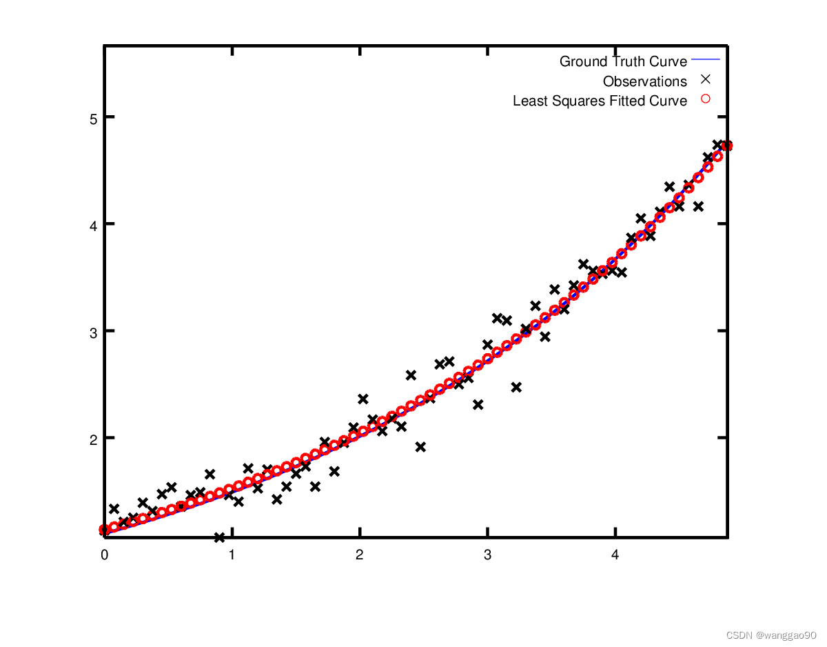
参数的初始值为m=0,c=0,初始代价函数为121.173。最后的解是m=0.291861,c=0.131439,代价是1.05675。
这个结果和期望解m=0.3,c=0.1有一些细微的差别,但是是合理的(因为添加了高斯噪声)。当从噪声数据重建曲线时,我们预计会看到这样的偏差。
实际上,如果您要对m=0.3,c=0.1的目标函数进行评估,那么当目标函数值为1.082425时,拟合效果会更差。下图说明了适合度。
2、Robust Curve Fitting
现在假设我们给出的数据有一些异常值(离群点/外点),也就是说,我们有一些点不服从噪声模型,继续使用上面的代码来拟合这些数据,我们将得到拟合曲线是偏离实际预期。
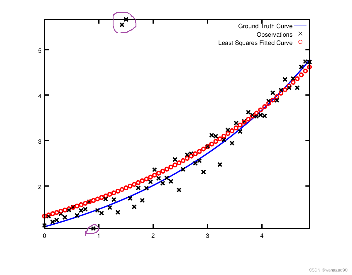
处理异常值的标准方法是使用LossFunction。损失函数降低了残差高的残差块(通常是与异常值对应的残差块)的影响。为了将损失函数与残差块联系起来,我们改变
// problem.AddResidualBlock(cost_function, nullptr , &m, &c);

problem.AddResidualBlock(cost_function, new CauchyLoss(0.5) , &m, &c);
这里使用SizedCostFunction类,需要填写计算jacobians。完整代码如下
#include "ceres/ceres.h"
#include "glog/logging.h"

// Data generated using the following octave code.
//   randn('seed', 23497);
//   m = 0.3;
//   c = 0.1;
//   x=[0:0.075:5];
//   y = exp(m * x + c);
//   noise = randn(size(x)) * 0.2;
//   outlier_noise = rand(size(x)) < 0.05;
//   y_observed = y + noise + outlier_noise;
//   data = [x', y_observed'];

const int kNumObservations = 67;
const double data[] = {


0.000000e+00, 1.133898e+00,
7.500000e-02, 1.334902e+00,
1.500000e-01, 1.213546e+00,
2.250000e-01, 1.252016e+00,
3.000000e-01, 1.392265e+00,
3.750000e-01, 1.314458e+00,
4.500000e-01, 1.472541e+00,
5.250000e-01, 1.536218e+00,
6.000000e-01, 1.355679e+00,
6.750000e-01, 1.463566e+00,
7.500000e-01, 1.490201e+00,
8.250000e-01, 1.658699e+00,
9.000000e-01, 1.067574e+00,
9.750000e-01, 1.464629e+00,
1.050000e+00, 1.402653e+00,
1.125000e+00, 1.713141e+00,
1.200000e+00, 1.527021e+00,
1.275000e+00, 1.702632e+00,
1.350000e+00, 1.423899e+00,
1.425000e+00, 5.543078e+00, // Outlier point
1.500000e+00, 5.664015e+00, // Outlier point
1.575000e+00, 1.732484e+00,
1.650000e+00, 1.543296e+00,
1.725000e+00, 1.959523e+00,
1.800000e+00, 1.685132e+00,
1.875000e+00, 1.951791e+00,
1.950000e+00, 2.095346e+00,
2.025000e+00, 2.361460e+00,
2.100000e+00, 2.169119e+00,
2.175000e+00, 2.061745e+00,
2.250000e+00, 2.178641e+00,
2.325000e+00, 2.104346e+00,
2.400000e+00, 2.584470e+00,
2.475000e+00, 1.914158e+00,
2.550000e+00, 2.368375e+00,
2.625000e+00, 2.686125e+00,
2.700000e+00, 2.712395e+00,
2.775000e+00, 2.499511e+00,
2.850000e+00, 2.558897e+00,
2.925000e+00, 2.309154e+00,
3.000000e+00, 2.869503e+00,
3.075000e+00, 3.116645e+00,
3.150000e+00, 3.094907e+00,
3.225000e+00, 2.471759e+00,
3.300000e+00, 3.017131e+00,
3.375000e+00, 3.232381e+00,
3.450000e+00, 2.944596e+00,
3.525000e+00, 3.385343e+00,
3.600000e+00, 3.199826e+00,
3.675000e+00, 3.423039e+00,
3.750000e+00, 3.621552e+00,
3.825000e+00, 3.559255e+00,
3.900000e+00, 3.530713e+00,
3.975000e+00, 3.561766e+00,
4.050000e+00, 3.544574e+00,
4.125000e+00, 3.867945e+00,
4.200000e+00, 4.049776e+00,
4.275000e+00, 3.885601e+00,
4.350000e+00, 4.110505e+00,
4.425000e+00, 4.345320e+00,
4.500000e+00, 4.161241e+00,
4.575000e+00, 4.363407e+00,
4.650000e+00, 4.161576e+00,
4.725000e+00, 4.619728e+00,
4.800000e+00, 4.737410e+00,
4.875000e+00, 4.727863e+00,
4.950000e+00, 4.669206e+00
};

using ceres::AutoDiffCostFunction;
using ceres::CostFunction;
using ceres::CauchyLoss;
using ceres::Problem;
using ceres::Solve;
using ceres::Solver;

class ExponentialResidual : public ceres::SizedCostFunction<1, 2> {


public:
    ExponentialResidual(double x, double y)
        : x_(x), y_(y) {

     }

    virtual bool Evaluate(const double* const* mc,
                          double* residual,
                          double** jacobians) const override
    {


        double tmp_y = exp(mc[0][0] * x_ + mc[0][1]);
        residual[0] = tmp_y - y_;   //  r = exp(mx+c) - y

        if(jacobians && jacobians[0]) {


            jacobians[0][0] = x_ * tmp_y;   // dr / dm
            jacobians[0][1] = tmp_y;        // dr / dc
        }

        return true;
    }

private:
    const double x_, y_;
};


int main(int argc, char** argv) {


  google::InitGoogleLogging(argv[0]);

  double mc[] = {

    0,0};

  double &m = mc[0];
  double &c = mc[1];

  Problem problem;
  for (int i = 0; i < kNumObservations; ++i) {


    problem.AddResidualBlock(new ExponentialResidual(data[2 * i], data[2 * i + 1]),
                             new CauchyLoss(0.5),  // 使用损失LossFunction,不再是nullptr
                             mc);
  }

  Solver::Options options;
  options.linear_solver_type = ceres::DENSE_QR;
  options.minimizer_progress_to_stdout = true;

  Solver::Summary summary;
  Solve(options, &problem, &summary);
  std::cout << summary.BriefReport() << "\n";
  std::cout << "Initial m: " << 0.0 << " c: " << 0.0 << "\n";
  std::cout << "Final   m: " << m << " c: " << c << "\n";
  return 0;
}
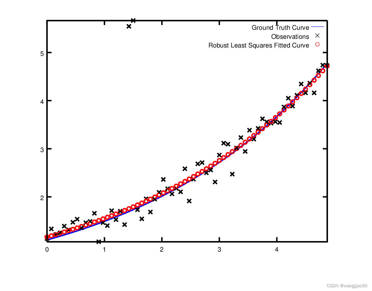
CauchyLoss 是Ceres Solver中的一个损失函数,参数0.5指定了损失函数的尺度。重新运行程序,得到的优化的结果相比不使用损失函数的结果更优。
iter      cost      cost_change  |gradient|   |step|    tr_ratio  tr_radius  ls_iter  iter_time  total_time
   0  1.815138e+01    0.00e+00    2.04e+01   0.00e+00   0.00e+00  1.00e+04        0    6.93e-04    1.14e-03
   1  2.259471e+01   -4.44e+00    0.00e+00   5.48e-01  -7.74e-01  5.00e+03        1    7.61e-04    2.26e-03
   2  2.258929e+01   -4.44e+00    0.00e+00   5.48e-01  -7.73e-01  1.25e+03        1    4.05e-04    2.74e-03
   3  2.255683e+01   -4.41e+00    0.00e+00   5.48e-01  -7.68e-01  1.56e+02        1    4.51e-04    5.16e-03
   4  2.225747e+01   -4.11e+00    0.00e+00   5.41e-01  -7.16e-01  9.77e+00        1    3.37e-04    5.58e-03
   5  1.784270e+01    3.09e-01    8.54e+01   4.72e-01   5.44e-02  5.72e+00        1    8.33e-04    6.48e-03
   6  7.557353e+00    1.03e+01    1.13e+02   1.06e-01   2.07e+00  1.72e+01        1    8.29e-04    7.38e-03
   7  2.674796e+00    4.88e+00    7.69e+01   5.41e-02   1.78e+00  5.15e+01        1    8.22e-04    8.28e-03
   8  1.946177e+00    7.29e-01    1.61e+01   5.00e-02   1.23e+00  1.54e+02        1    8.22e-04    9.17e-03
   9  1.904587e+00    4.16e-02    2.20e+00   2.64e-02   1.11e+00  4.63e+02        1    8.23e-04    1.01e-02
  10  1.902929e+00    1.66e-03    2.28e-01   6.94e-03   1.12e+00  1.39e+03        1    8.93e-04    1.10e-02
  11  1.902884e+00    4.51e-05    1.49e-02   1.27e-03   1.14e+00  4.17e+03        1    9.34e-04    1.21e-02
Ceres Solver Report: Iterations: 12, Initial cost: 1.815138e+01, Final cost: 1.902884e+00, Termination: CONVERGENCE
Initial m: 0 c: 0
Final   m: 0.287605 c: 0.151213
3、Circle Fitting 代价函数定义问题
3.1、代价函数定义
对于 2D 圆的一般方程为:
( x − a ) 2 + ( y − b ) 2 = r 2 (x-a)^2 + (y-b)^2 = r^2 (x−a)2+(y−b)2=r2
式中 ( a , b ) (a,b) (a,b)为圆心, r r r为半径。
假设有 k 个 2D 观测点数据 k ( x i , y i ) , i = 1 , 2 , . . . , k k(x_i,y_i),i = 1,2,...,k k(xi,yi),i=1,2,...,k,根据观测点数据拟合圆,并获取拟合圆的圆心$ (a,b)$ 和半径 r r r ,可以先构建如下非线性最小二乘问题:
m i n 1 2 ∑ i = 1 k ∣ ∣ f ( a , b , r ) ∣ ∣ 2 min \frac{1}{2}\displaystyle\sum_{i=1}^k ||f(a,b,r)||^2 min21i=1∑k∣∣f(a,b,r)∣∣2
后面说明集中代价函数 f ( a , b , r ) f(a,b,r) f(a,b,r)的定义
-
第一种定义
最直观的理解代价函数是,观测点到圆心的距离,
f ( a , b , r ) = r − ( x i − a ) 2 + ( y i − b ) 2 f(a,b,r) = r - \sqrt{(x_i -a)^2 + (y_i-b)^2} f(a,b,r)=r−(xi−a)2+(yi−b)2看似比较直观、合理,但其中的根号运算让代价函数更加非线性,求解效率不高 -
第二种定义
直接在圆定义上调整如下
f ( a , b , r ) = r 2 − [ ( x i − a ) 2 + ( y i − b ) 2 ] f(a,b,r) = r^2 - [(x_i -a)^2 + (y_i-b)^2] f(a,b,r)=r2−[(xi−a)2+(yi−b)2] 虽然严格意义上不能表示点到圆心的距离,但通常更加鲁棒(尤其是存在外点时),这是因为代价函数更符合凸函数,更容易找到期望的最小值。 -
第三种定义
在第二种方案中,估计出来的半径 r r r 可能是负值,与实际不符,需要增加约束,重新构建非线性最小二乘问题,有如下方案:
令 r 2 = r 2 r_2 = r^2 r2=r2, 待估计的参数将变成 ( a , b , r 2 ) (a,b,r_2) (a,b,r2), 代价函数如下:
f ( a , b , r 2 ) = r 2 − [ ( x i − a ) 2 + ( y i − b ) 2 ] f(a,b,r_2) = r_2 - [(x_i -a)^2 + (y_i-b)^2] f(a,b,r2)=r2−[(xi−a)2+(yi−b)2]此时估计出的 r 2 r_2 r2 肯定是正值,实际求解的 r = r 2 r = \sqrt{r_2} r=r2也是正值。
3.2、示例代码
我们期望拟合的圆为 ( x − 2 ) 2 + ( y − 2 ) 2 = 3 2 (x-2)^2+(y-2)^2 = 3^2 (x−2)2+(y−2)2=32,我们随机生成一堆点,故意设定初值为 ( 8 , 8 , − 1 ) (8, 8, -1) (8,8,−1),比较两种结果。直接给出解析解的方式。
3.2.1 代码1
先以第二种方案,
class DistanceFromCircleCost : public ceres::SizedCostFunction<1,1,1,1>{


public:
    DistanceFromCircleCost(double xx, double yy) : xx_(xx), yy_(yy) {

    }

    virtual bool Evaluate(double const* const* parameters,
                          double* residuals,
                          double** jacobians) const override
    {


        // circle: f(x,y) = (x-x0)^2 + (y-y0)^2 - r^2
        double dx = xx_ - parameters[0][0];
        double dy = yy_ - parameters[1][0];
        double r_squar = parameters[2][0] * parameters[2][0];
        residuals[0] = pow(dx, 2) + pow(dy, 2) - r_squar;

        if(jacobians && jacobians[0]) {


            jacobians[0][0] = - 2 * dx;
            jacobians[0][1] = - 2 * dy;
            jacobians[0][2] = - 2 * parameters[2][0];
        }

        return true;
    }

private:
    const double xx_, yy_;
};

int main(int argc, char** argv)
{


    double x = 8;
    double y = -8;
    double r = -1;

    double initial_x = x;
    double initial_y = y;
    double initial_r = r;

    Problem problem;
    LossFunction* loss = new CauchyLoss(0.1);

    // 优化圆  (x-2)^2+(y-2)^2 = 3^2
    double estimate_x = 2;
    double estimate_y = 2;
    double estimate_r = 3;

    for(double ang = 0; ang < 360; ang += 2) {


        double rad = ang * 3.1415925 / 180;
        double xx = estimate_x + estimate_r *cos(rad) + (rand() % 10 - 5) / 50.;
        double yy = estimate_y + estimate_r *sin(rad) + (rand() % 10 - 5) / 50.;

        problem.AddResidualBlock(
            new ceres::NumericDiffCostFunction<DistanceFromCircleCost, ceres::CENTRAL, 1,1,1,1>(
                new DistanceFromCircleCost(xx, yy)),
            loss,
            &x, &y, &r
        );
    }


    // Build and solve the problem.
    Solver::Options options;
    options.max_num_iterations = 500;
    options.linear_solver_type = ceres::DENSE_QR;
    options.minimizer_progress_to_stdout = true;
    Solver::Summary summary;
    Solve(options, &problem, &summary);

    std::cout << summary.BriefReport() << "\n";
    std::cout << "x : " << initial_x << " -> " << x << "\n";
    std::cout << "y : " << initial_y << " -> " << y << "\n";
    std::cout << "r : " << initial_r << " -> " << r << "\n";
    return 0;
}
结果如下,显然求解半径为负值不符合。
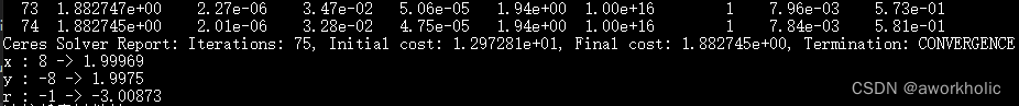
3.2.2 代码2
class DistanceFromCircleCost : public ceres::SizedCostFunction<1,1,1,1>{


public:
    DistanceFromCircleCost(double xx, double yy) : xx_(xx), yy_(yy) {

    }

    virtual bool Evaluate(double const* const* parameters,
                          double* residuals,
                          double** jacobians) const override
    {


        // circle: f(x,y) = (x-x0)^2 + (y-y0)^2 - r^2
        double dx = xx_ - parameters[0][0];
        double dy = yy_ - parameters[1][0];
        double r_squar = parameters[2][0];
        residuals[0] = pow(dx, 2) + pow(dy, 2) - r_squar;

        if(jacobians && jacobians[0]) {


            jacobians[0][0] = - 2 * dx;
            jacobians[0][1] = - 2 * dy;
            jacobians[0][2] = -1;
        }

        return true;
    }

private:
    const double xx_, yy_;
};

int main(int argc, char** argv)
{


    double x = 8;
    double y = -8;
    double r = -2;

    double initial_x = x;
    double initial_y = y;
    double initial_r = r;

    Problem problem;
    LossFunction* loss = new CauchyLoss(0.1);

    // 优化圆  (x-2)^2+(y-2)^2 = 3^2
    double estimate_x = 2;
    double estimate_y = 2;
    double estimate_r = 3;

    double estimate_r_squar = estimate_r * estimate_r;

    for(double ang = 0; ang < 360; ang += 2) {


        double rad = ang * 3.1415925 / 180;
        double xx = estimate_x + estimate_r *cos(rad) + (rand() % 10 - 5) / 50.;
        double yy = estimate_y + estimate_r *sin(rad) + (rand() % 10 - 5) / 50.;

        problem.AddResidualBlock(
            new ceres::NumericDiffCostFunction<DistanceFromCircleCost, ceres::CENTRAL, 1,1,1,1>(
                new DistanceFromCircleCost(xx, yy)),
            loss,
            &x, &y, &estimate_r_squar
        );
    }


    // Build and solve the problem.
    Solver::Options options;
    options.max_num_iterations = 500;
    options.linear_solver_type = ceres::DENSE_QR;
    options.minimizer_progress_to_stdout = true;
    Solver::Summary summary;
    Solve(options, &problem, &summary);

    std::cout << summary.BriefReport() << "\n";
    std::cout << "x : " << initial_x << " -> " << x << "\n";
    std::cout << "y : " << initial_y << " -> " << y << "\n";
    std::cout << "r : " << initial_r << " -> " << sqrt(estimate_r_squar) << "\n";
    return 0;
}
运行结果如下,正确
