一、前言

Python 是一种能够执行水文研究和水资源评估计算的编程语言。 我们使用 Python 和数字/空间库（如 Numpy 和 Rasterio）完成了波多黎各帕蒂拉斯湖的体积-高程曲线确定教程。 最后，将结果与 USGS 调查中的体积-海拔曲线进行了比较。

这次是针对湖泊完成的程序，但当底部高程作为栅格文件可用时，可以轻松应用于任何水库或水体。

二、实现过程

（1）导入相应的库

import rasterio
import numpy as np
import pandas as pd
import matplotlib.pyplot as plt
from mpl_toolkits.axes_grid1 import make_axes_locatable

（2）打开影像

lakeRst = rasterio.open('../Rst/lakeBottomElevation.tif')
lakeRst.count
1
#raster resolution
lakeRst.res
(0.5, 0.5)
#all raster crs info
lakeRst.crs.wkt
'PROJCS["NAD83(2011) / Puerto Rico and Virgin Is.",GEOGCS["NAD83(2011)",DATUM["NAD83_National_Spatial_Reference_System_2011",SPHEROID["GRS 1980",6378137,298.257222101,AUTHORITY["EPSG","7019"]],AUTHORITY["EPSG","1116"]],PRIMEM["Greenwich",0,AUTHORITY["EPSG","8901"]],UNIT["degree",0.0174532925199433,AUTHORITY["EPSG","9122"]],AUTHORITY["EPSG","6318"]],PROJECTION["Lambert_Conformal_Conic_2SP"],PARAMETER["latitude_of_origin",17.8333333333333],PARAMETER["central_meridian",-66.4333333333333],PARAMETER["standard_parallel_1",18.4333333333333],PARAMETER["standard_parallel_2",18.0333333333333],PARAMETER["false_easting",200000],PARAMETER["false_northing",200000],UNIT["metre",1,AUTHORITY["EPSG","9001"]],AXIS["Easting",EAST],AXIS["Northing",NORTH],AUTHORITY["EPSG","6566"]]'

（3）获取栅格值作为 Numpy 数组

lakeBottom = lakeRst.read(1)
#raster sample
lakeBottom[:5,:5]
array([[-3.4028235e+38, -3.4028235e+38, -3.4028235e+38, -3.4028235e+38,
        -3.4028235e+38],
       [-3.4028235e+38, -3.4028235e+38, -3.4028235e+38, -3.4028235e+38,
        -3.4028235e+38],
       [-3.4028235e+38, -3.4028235e+38, -3.4028235e+38, -3.4028235e+38,
        -3.4028235e+38],
       [-3.4028235e+38, -3.4028235e+38, -3.4028235e+38, -3.4028235e+38,
        -3.4028235e+38],
       [-3.4028235e+38, -3.4028235e+38, -3.4028235e+38, -3.4028235e+38,
        -3.4028235e+38]], dtype=float32)
#replace value for np.nan
noDataValue = np.copy(lakeBottom[0,0])

lakeBottom[lakeBottom==noDataValue]= np.nan
plt.figure(figsize=(12,12))
plt.imshow(lakeBottom)
plt.show()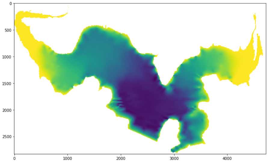

（4）湖泊体积计算

# get raster minimum and maximum 
minElev = np.nanmin(lakeBottom)
maxElev = np.nanmax(lakeBottom)
print('Min bottom elevation %.2f m., max bottom elevation %.2f m.'%(minElev,maxElev))

# steps for calculation
nSteps = 20

# lake bottom elevation intervals
elevSteps = np.round(np.linspace(minElev,maxElev,nSteps),2)
elevSteps
Min bottom elevation 44.10 m., max bottom elevation 67.55 m.





array([44.1 , 45.33, 46.56, 47.8 , 49.03, 50.27, 51.5 , 52.74, 53.97,
       55.21, 56.44, 57.67, 58.91, 60.14, 61.38, 62.61, 63.85, 65.08,
       66.32, 67.55])
# definition of volume function
def calculateVol(elevStep,elevDem,lakeRst):
    tempDem = elevStep - elevDem[elevDem<elevStep]
    tempVol = tempDem.sum()*lakeRst.res[0]*lakeRst.res[1]
    return tempVol
# calculate volumes for each elevation
volArray = []
for elev in elevSteps:
    tempVol = calculateVol(elev,lakeBottom,lakeRst)
    volArray.append(tempVol)

print("Lake bottom elevations %s"%elevSteps)
volArrayMCM = [round(i/1000000,2) for i in volArray]
print("Lake volume in million of cubic meters %s"%volArrayMCM)
Lake bottom elevations [44.1  45.33 46.56 47.8  49.03 50.27 51.5  52.74 53.97 55.21 56.44 57.67
 58.91 60.14 61.38 62.61 63.85 65.08 66.32 67.55]
Lake volume in million of cubic meters [0.0, 0.0, 0.13, 0.38, 0.68, 1.02, 1.4, 1.83, 2.31, 2.88, 3.56, 4.3, 5.1, 5.97, 6.91, 7.92, 8.99, 10.12, 11.3, 12.54]
# plot values
fig, ax = plt.subplots(figsize=(12,5))
ax.plot(volArrayMCM,elevSteps,label='Patillas lake')
ax.grid()
ax.legend()
ax.set_xlabel('Volume MCM')
ax.set_ylabel('Elevation (masl)')
plt.show()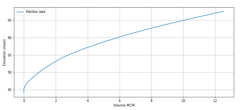

# plot values
fig, [ax1, ax2] = plt.subplots(1,2,figsize=(20,8),gridspec_kw={'width_ratios': [2, 1]})
ax1.set_title('Lake bottom elevation')
botElev = ax1.imshow(lakeBottom)

divider = make_axes_locatable(ax1)
cax = divider.append_axes('bottom', size='5%', pad=0.5)
fig.colorbar(botElev, cax=cax, orientation='horizontal', label='Elevation (masl)') 

ax2.plot(volArrayMCM,elevSteps,label='Patillas lake')
ax2.grid()
ax2.legend()
ax2.set_xlabel('Volume MCM')
ax2.set_ylabel('Elevation (masl)')
plt.show()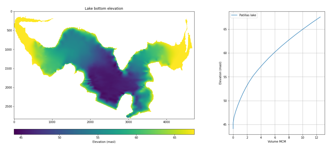

（5）与美国地质勘探局调查的比较

patVol = pd.read_csv('../Txt/patillasVolume.csv')
patVol.head()

fig, ax = plt.subplots(figsize=(12,5))
ax.plot(volArrayMCM,elevSteps,label='Patillas lake',ls= '-.')
ax.plot(patVol['Storage_capacity_mcm'],patVol['Pool_Elevation_m'],label='Patillas lake - USGS Survey')
ax.grid()
ax.legend()
ax.set_xlabel('Volume MCM')
ax.set_ylabel('Elevation (masl)')
Text(0, 0.5, 'Elevation (masl)')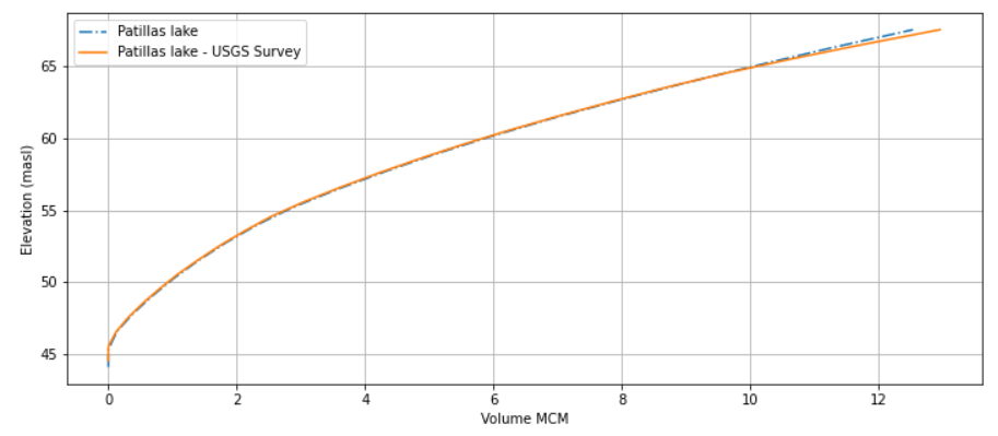

数据下载地址：https://hatarilabs.com/s/howToMakeALakeVolumeElevationCurvePython.rar