本文在博主 shyern 博文的基础上旨在介绍 STGCN 的原理及其实现，使用 tensorflow 2 实现了 STGCN 的基本操作。

作者通过将图卷积网络扩展到时空图模型，设计了一种（用于动作识别的骨架序列）的通用表示，叫做时空图卷积网络（Spatio-Temporal Graph Convolutional Networks，STGCN）。

Graph Construction

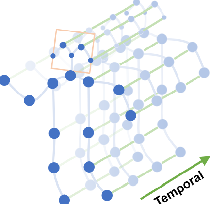
记一个有 $N$ 个节点和 $T$ 帧的骨骼序列的时空图为 $G=(V,E)$ ，其节点集合为 V = { v t i ∣ t = 1 , … , T , i = 1 , . . . , N } V=\left\{v_{t i} | t=1, \ldots, T, i=1,...,N\right\} V={ vti​∣t=1,…,T,i=1,...,N} ，第 $t$ 帧的第 $i$ 个节点的特征向量 $F\left(v_{ti}\right)$ 由该节点的坐标向量和估计置信度组成。

图结构由两个部分组成：

• 根据人体结构，将每一帧的节点连接成边，这些边形成 spatial edges

  E S = { v t i v t j ∣ ( i , j ) ∈ H } E_{S}=\left\{v_{t i} v_{t j} |(i, j) \in H\right\} ES​={ vti​vtj​∣(i,j)∈H}

  $H$ 是一组自然连接的人体关节。

• 将连续两帧中相同的节点连接成边，这些边形成temporal edges

  $$E_F=\left\{v_{ti}{v}_{(t+1)i}\right\}$$

Spatial Graph Convolutional Neural Network

对于空间图卷积，在这里只针对某一帧讨论图卷积模型操作。以常见的图像的二维卷积为例，针对某一位置 $\mathbf{x}$ 的卷积输出可以写成如下形式

$$f_{out}(\mathbf{x})=\sum _{h=1}^K\sum _{w=1}^K{f}_{in}(\mathbf{p}(\mathbf{x},h,w))\cdot \mathbf{w}\cdot \mathbf{w}(h,w)$$

输入通道数为 $c$ 的特征图 $f_{in}$ ，卷积核大小 $K\times K$ ，sampling
function 采样函数 $\mathbf{p}(\mathbf{x},h,w)=\mathbf{x}+{\mathbf{p}}^{\prime }(h,w)$ ， weight function 通道数为 $c$ 的权重函数。

• Sampling function

在图像中，采样函数 $\mathbf{p}(h,w)$ 指的是以 $x$ 像素为中心的周围邻居像素，在图中，邻居像素集合被定义为：

B ( v t i ) = { v t j ∣ d ( v t j , v t i ) ≤ D } B\left(v_{t i}\right)=\left\{v_{t j} | d\left(v_{t j}, v_{t i}\right) \leq D\right\} B(vti​)={ vtj​∣d(vtj​,vti​)≤D}

其中， $d(v_{tj},v_{ti})$ 指的是从 $v_{tj}$ 到 $v_{ti}$ 的最短距离，因此采样函数可以写成

$$\mathbf{p}\left(v_{ti},v_{tj}\right)=v_{tj}$$

• Weight function

在 2D 卷积中，邻居像素规则地排列在中心像素周围，因此可以根据空间顺序用规则的卷积核对其进行卷积操作。类比2D卷积，在图中，将 sampling function 得到的邻居像素划分成不同的子集，每一个子集有一个数字标签，因此有

l t i : B ( v t i ) → { 0 , … , K − 1 } l_{t i} : B\left(v_{t i}\right) \rightarrow\{0, \ldots, K-1\} lti​:B(vti​)→{ 0,…,K−1}

将一个邻居节点映射到对应的子集标签，权重方程为

$$\mathbf{w}\left(v_{ti},v_{tj}\right)={\mathbf{w}}^{\prime }\left(l_{ti}\left(v_{tj}\right)\right)$$

• Spatial Graph convolution

$$f_{out}\left(v_{ti}\right)=\sum _{v_{tj}\in B\left(v_{ti}\right)}\frac{1}{Z_{ti}\left(v_{tj}\right)}{f}_{in}\left(\mathbf{p}\left(v_{ti},v_{tj}\right)\right)\cdot \mathbf{w}\left(v_{ti},v_{tj}\right)$$

其中归一化项

Z t i ( v t j ) = ∣ { v t k ∣ l t i ( v t k ) = l t i ( v t j ) } ∣ Z_{t i}\left(v_{t j}\right)=\left|\left\{v_{t k} | l_{t i}\left(v_{t k}\right)=l_{t i}\left(v_{t j}\right)\right\}\right| Zti​(vtj​)=∣{ vtk​∣lti​(vtk​)=lti​(vtj​)}∣

等价于对应子集的基。将上述公式带入上式得到：

$$f_{out}\left(v_{ti}\right)=\sum _{v_{tj}\in B\left(v_{ti}\right)}\frac{1}{Z_{ti}\left(v_{tj}\right)}{f}_{in}\left(v_{tj}\right)\cdot \mathbf{w}\left(l_{ti}\left(v_{tj}\right)\right)$$

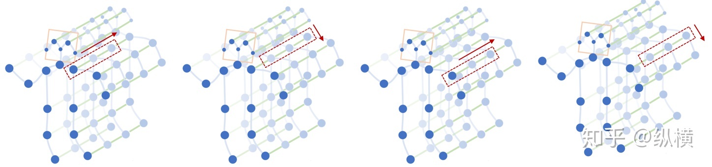
• Spatial Temporal Modelling

将空间域的模型扩展到时间域中，得到的 sampling function 为

B ( v t i ) = { v q j ∣ d ( v t j , v t i ) ≤ K , ∣ q − t ∣ ≤ ⌊ Γ / 2 ⌋ } B\left(v_{t i}\right)=\left\{v_{q j}\left|d\left(v_{t j}, v_{t i}\right) \leq K,\right| q-t | \leq\lfloor\Gamma / 2\rfloor\right\} B(vti​)={ vqj​∣d(vtj​,vti​)≤K,∣q−t∣≤⌊Γ/2⌋}

其中，$\Gamma$ 控制控制时间域的卷积核大小。

weight function 为

$$l_{ST}\left(v_{qj}\right)=l_{ti}\left(v_{tj}\right)+(q-t+\lfloor \Gamma /2\rfloor )\times K$$

其中，$l_{ii}$ 为单帧情况的标签映射。

至此，在构造的时空图上有一个定义明确的卷积运算。

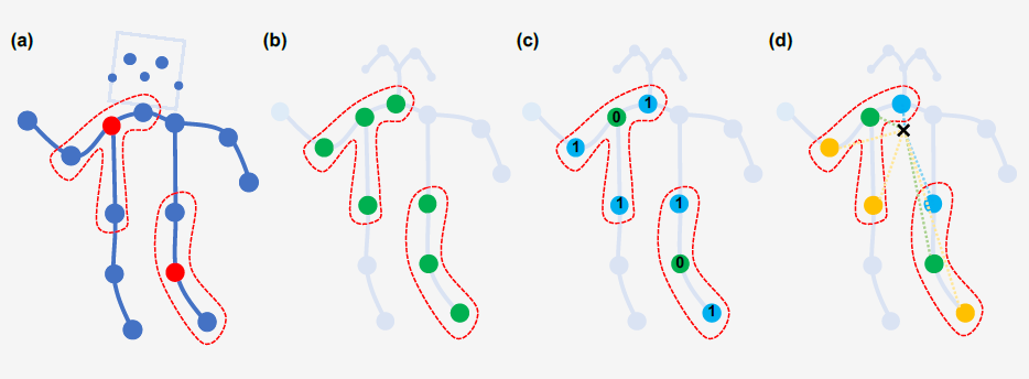
Partition Strategies

• 唯一划分 Uni-labelling：将节点的1邻域划分为一个子集
• 基于距离的划分 Distance partitioning：将节点的1邻域划分为两个子集，节点本身子集与邻节点子集
• 空间构型划分 Spatial configuration partitioning：将节点的1邻域划分为 3 个子集，第一个子集连接了空间位置上比根节点更远离整个骨架的邻居节点，第二个子集连接了更靠近中心的邻居节点，第三个子集为根节点本身，分别表示了离心运动、向心运动和静止的运动特征

Learnable edge importance weighting

在运动过程中，不同的躯干重要性是不同的。例如腿的动作可能比脖子重要，通过腿部我们甚至能判断出跑步、走路和跳跃，但是脖子的动作中可能并不包含多少有效信息。

因此，STGCN 对不同躯干进行了加权（每个 STGCN 单元都有自己的权重参数用于训练）。增加注意力机制后

$${\mathbf{A}}_j={\mathbf{A}}_j\otimes \mathbf{M}$$

其中，$\otimes$ 表示点积，mask $\mathbf{M}$ 被初始化为 tf.ones。

Implementing STGCN

GCN 帮助我们学习了到空间中相邻关节的局部特征。在此基础上，我们需要学习时间中关节变化的局部特征。**如何为 Graph 叠加时序特征，是图网络面临的问题之一。**这方面的研究主要有两个思路：时间卷积（TCN）和序列模型（LSTM）。

STGCN 使用的是 TCN，由于形状固定，我们可以使用传统的卷积层完成时间卷积操作。为了便于理解，可以类比图像的卷积操作。

$${\mathbf{f}}_{out}={\mathbf{\Lambda }}^{-\frac{1}{2}}(\mathbf{A}+\mathbf{I}){\mathbf{\Lambda }}^{-\frac{1}{2}}{\mathbf{f}}_{in}\mathbf{W}$$

其中，${\Lambda }^{ii}={\sum }_j\left(A^{ij}+I^{ij}\right)$。

注意：作者使用 pytorch 实现，故其 tensor shape 为 $(N,C,H,W)$，而本文使用的 tensorflow 的 tensor shape 为 $(N,H,W,C)$ 。有兴趣的读者可以对比二者的区别，以下表述采用后者。

STGCN 的 feature map 最后三个维度的形状为 $(T,V,C)$ ，与图像 feature map 的形状 $(H,W,C)$ 相对应。

• 图像的通道数 $C$ 对应关节的特征数 $C$
• 图像的宽 $W$ 对应关键帧数 $V$
• 图像的高 $H$ 对应关节数 $T$

Spatial graph convolution model

在空间图卷积中，卷积核的大小为 $w\times 1$，则每次完成 w 行像素，1 列像素的卷积。stride 为 $s$，则每次移动 $s$ 像素，完成 1 行后进行下 1 行像素的卷积。

# The based unit of graph convolution networks.
import tensorflow as tf

from tensorflow.keras.models import Model
from tensorflow.keras.layers import Conv2D, Reshape

class gcn(Model):
    r"""The basic module for applying a graph convolution.

    Args:
        filters (int): Number of channels produced by the convolution
        kernel_size (int): Size of the graph convolution kernel
        t_kernel_size (int): Size of the temporal convolution kernel
        t_stride (int, optional): Stride of the temporal convolution. Default: 1
        t_padding (int, optional): Temporal zero-padding added to both sides of
            the input. Default: 0
        t_dilation (int, optional): Spacing between temporal kernel elements.
            Default: 1
        bias (bool, optional): If ``True``, adds a learnable bias to the output.
            Default: ``True``

    Shape:
        - Input[0]: Input graph sequence in :math:`(N, T_{in}, V, in_channels)` format
        - Input[1]: Input graph adjacency matrix in :math:`(K, V, V)` format
        - Output[0]: Output graph sequence in :math:`(N, T_{out}, V, out_channels)` format
        - Output[1]: Graph adjacency matrix for output data in :math:`(K, V, V)` format

        where
            :math:`N` is a batch size,
            :math:`T_{in}/T_{out}` is a length of input/output sequence,
            :math:`V` is the number of graph nodes,
            :math:`K` is the spatial kernel size, as :math:`K == kernel_size[1]`.
    """

    def __init__(self,
                 filters,
                 t_kernel_size=1,
                 t_stride=1,
                 t_padding=0,
                 t_dilation=1,
                 bias=True):
        super(gcn, self).__init__(dynamic=True)

        self.filters = filters
        self.t_kernel_size = t_kernel_size // 2 * 2 + 1
        self.t_padding = t_padding
        self.t_stride = t_stride
        self.t_dilation = t_dilation
        self.bias = bias
        self.k_size = None

        self.conv = None
        self.reshape = None

    def build(self, input_shape):
        x_shape, A_shape = input_shape

        self.k_size = A_shape[0]
        self.conv = Conv2D(
            filters=self.filters * self.k_size,
            kernel_size=(self.t_kernel_size, 1),
            padding='same' if self.t_padding else 'valid',
            strides=(self.t_stride, 1),
            dilation_rate=(self.t_dilation, 1),
            use_bias=self.bias,
            input_shape=x_shape)

        n, t, v, c = self.conv.compute_output_shape(x_shape)
        self.reshape = Reshape([t, v, self.k_size, c // self.k_size])

    def call(self, inputs, training=None, mask=None):
        x, A = inputs

        h = self.conv(x)
        h = self.reshape(h)
        y = tf.einsum('ntvkc, kvw->ntwc', h, A)

        return y

Temporal convolution model

在时间卷积中，卷积核的大小为 $temporal\_kernel\_size\times 1$ ，则每次完成 1 个节点，temporal_kernel_size 个关键帧的卷积。$s$ 为 1，则每次移动 1 帧，完成 1 个节点后进行下 1 个节点的卷积。

# The based unit of graph temporal convolution networks.

from tensorflow.keras.models import Model
from tensorflow.keras.layers import Conv2D, Dropout, BatchNormalization, Lambda, Activation

class tcn(Model):
    r"""The basic module for applying a temporal convolution.

    Args:
        input_A (float): Graph adjacency matrix for output data in :math:`(K, V, V)` format
        filters (int): Number of channels produced by the convolution
        kernel_size (int): Size of the graph convolution kernel
        t_kernel_size (int): Size of the temporal convolution kernel
        t_stride (int, optional): Stride of the temporal convolution. Default: 1
        t_padding (int, optional): Temporal zero-padding added to both sides of
            the input. Default: 0
        t_dilation (int, optional): Spacing between temporal kernel elements.
            Default: 1
        bias (bool, optional): If ``True``, adds a learnable bias to the output.
            Default: ``True``

    Shape:
        - Input[0]: Input graph sequence in :math:`(N, T_{in}, V, in_channels)` format
        - Output[0]: Output graph sequence in :math:`(N, T_{out}, V, out_channels)` format

        where
            :math:`N` is a batch size,
            :math:`T_{in}/T_{out}` is a length of input/output sequence,
            :math:`V` is the number of graph nodes,
            :math:`K` is the spatial kernel size, as :math:`K == kernel_size[1]`.
    """

    def __init__(self,
                 filters,
                 t_kernel_size=1,
                 t_stride=1,
                 t_padding=0,
                 in_batchnorm=True,
                 out_batchnorm=True,
                 t_dilation=1,
                 bias=True,
                 dropout=0):
        super(tcn, self).__init__()

        self.filters = filters
        self.t_kernel_size = t_kernel_size
        self.t_padding = t_padding
        self.t_stride = t_stride
        self.t_dilation = t_dilation
        self.dropout = dropout
        self.bias = bias

        if in_batchnorm:
            self.batch_1 = BatchNormalization()
        else:
            self.batch_1 = Lambda(lambda x: x)

        self.conv = None
        self.a = Activation('relu')

        if out_batchnorm:
            self.batch_2 = BatchNormalization()
        else:
            self.batch_2 = Lambda(lambda x: x)

        self.dropout = Dropout(dropout)

    def build(self, input_shape):
        self.conv = Conv2D(filters=self.filters,
                           kernel_size=(self.t_kernel_size, 1),
                           padding='same' if self.t_padding else 'valid',
                           strides=(self.t_stride, 1),
                           dilation_rate=(self.t_dilation, 1),
                           use_bias=self.bias,
                           input_shape=input_shape)


    def call(self, inputs, training=None, mask=None):
        x = inputs

        h = self.batch_1(x)
        h = self.a(h)
        h = self.conv(h)
        h = self.batch_2(h)
        y = self.dropout(h)

        return y

Network architecture

输入的数据首先进行 batch normalization，然后在经过 9 个 STGCN 单元，接着是一个 global pooling 得到每个序列的 256 维特征向量，最后用 SoftMax 函数进行分类，得到最后的标签。每一个 STGCN 采用 Resnet 的结构，前三层的输出有 64 个通道，中间三层有128 个通道，最后三层有 256 个通道，在每次经过ST-CGN结构后，以0.5的概率随机将特征 dropout，第4和第7个时域卷积层的strides设置为2。用 SGD 训练，学习率为 0.01，每 10 个epochs学习率下降0.1。

本文实现了一个基本的 STGCN 单元，有兴趣的读者可以利用该单元进行时空图网络的设计并应用到实际的任务中。

# The based unit of spatial temporal module.

from tensorflow.keras.models import Model
from tensorflow.keras.layers import Activation, Lambda

from models.gcn import gcn
from models.tcn import tcn
from models.res import res

class stgcn(Model):
    r"""Applies a spatial temporal graph convolution over an input graph sequence.

    Args:
        filters (int): Number of channels produced by the convolution
        kernel_size (tuple): Size of the temporal convolution kernel
                                & graph convolution kernel
        stride (int, optional): Stride of the temporal convolution. Default: 1
        dropout (int, optional): Dropout rate of the final output. Default: 0
        residual (bool, optional): If ``True``, applies a residual mechanism.
                                Default: ``True``

    Shape:
        - Input[0]: Input graph sequence in :math:`(N, in_channels, T_{in}, V)` format
        - Input[1]: Input graph adjacency matrix in :math:`(K, V, V)` format
        - Output[0]: Output graph sequence in :math:`(N, out_channels, T_{out}, V)` format

        where
            :math:`N` is a batch size,
            :math:`T_{in}/T_{out}` is a length of input/output sequence,
            :math:`V` is the number of graph nodes,
            :math:`K` is the spatial kernel size, as :math:`K == kernel_size[1]`.

    """
    def __init__(self,
                 filters,
                 kernel_size,
                 stride=1,
                 dropout=0,
                 residual=True):
        super(stgcn, self).__init__(dynamic=True)

        assert len(kernel_size) == 2
        assert kernel_size[0] % 2 == 1
        padding = (kernel_size[0] - 1) // 2

        self.residual = residual
        self.filters = filters
        self.kernel_size = kernel_size
        self.res = None
        self.stride = stride

        self.gcn = gcn(filters=filters,
                       t_kernel_size=kernel_size[1])

        self.tcn = tcn(filters=filters,
                       t_kernel_size=kernel_size[0],
                       t_stride=stride,
                       t_padding=padding,
                       dropout=dropout)

        self.a = Activation('relu')

    def build(self, input_shape):
        x_shape, _ = input_shape
        c = x_shape[-1]

        if not self.residual:
            self.res = Lambda(lambda x: 0)
        elif c == self.filters and self.stride == 1:
            self.res = Lambda(lambda x: x)
        else:
            self.res = res(filters=self.filters,
                           kernel_size=1,
                           stride=self.stride)

    def call(self, inputs, training=None, mask=None):
        x, A = inputs

        res = self.res(x)
        x = self.gcn([x, A])
        x = self.tcn(x) + res
        y = self.a(x)

        return y

总结

GCN 在时间、空间上的拓展应用，作者采用 pytorch 实现，思路值得学习。本文借鉴使用 tensorflow 2 实现了基本的STGCN 单元，希望能偶基于作者的思路开发出更多版 STGCN，并用于具体的领域问题。