支持向量机(SVM)是一种流行的分类技术。虽然提出时间到现在有70来年了,但在90年代获得了很好的发展和扩展,在人像识别、文本分类、手写字符识别、生物信息学等模式识别问题中有得到应用。然而,对于不熟悉SVM的初学者来说,往往会因为错过了一些简单但重要的步骤而得到不理想的结果。
LIBSVM(A Library for Support Vector Machines)支持向量机库,是台湾大学林智仁(Lin Chih-Jen)教授等开发设计的一个简单、易于使用和快速有效的SVM模式识别与回归的软件包,是目前使用最广泛的支持向量机(SVM)包。包含标准SVM算法、概率输出、支持向量回归、多分类SVM等功能,其源代码由C编写,并有JAVA、Python、R、MATLAB等语言的调用接口、基于CUDA的GPU加速和其它功能性组件,例如多核并行计算、模型交叉验证等
1、安装SVM库
同样的,可以新建一个虚拟环境来进行全新安装
conda create -n mylibsvm python=3.7
激活环境
activate mylibsvm
安装时,依然建议带上豆瓣镜像,速度快
pip install libsvm-official -i http://pypi.douban.com/simple/ --trusted-host pypi.douban.com
pip install -U liblinear-official -i http://pypi.douban.com/simple/ --trusted-host pypi.douban.com
2、heart_scale数据集
2.1、下载并对数据集内容格式的熟悉
数据集的内容需符合LIBSVM格式的要求,实质是一个文本文件,我们打开看下,如图:
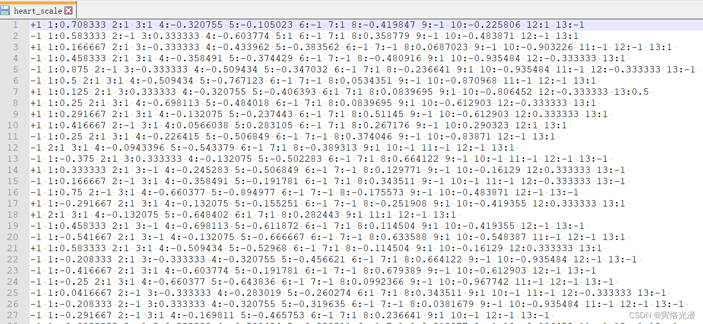 下载地址(里面还包括了自己制作数据集,后面有介绍):heart_scale数据集
2.2、训练并预测
代码都比较简单,导入libsvm库,加载数据集,进行训练即可
from libsvm.svmutil import *
y, x = svm_read_problem('heart_scale')
m = svm_train(y[:200], x[:200], '-c 4')
'''
*.*
optimization finished, #iter = 257
nu = 0.351161
obj = -225.628984, rho = 0.636110
nSV = 91, nBSV = 49
Total nSV = 91
'''
看下预测的效果,总共是270个样本!
p_label, p_acc, p_val = svm_predict(y, x, m) #全部预测
#Accuracy = 89.2593% (241/270) (classification)

p_label, p_acc, p_val = svm_predict(y[10:], x[10:], m)#第10个开始预测
#Accuracy = 89.6154% (233/260) (classification)其中svm_train第三个可选参数,内容如下(当然自己也可以help(svm_train)看到):
options:
-s svm_type : set type of SVM (default 0)
0 -- C-SVC (multi-class classification)
1 -- nu-SVC (multi-class classification)
2 -- one-class SVM
3 -- epsilon-SVR (regression)
4 -- nu-SVR (regression)
-t kernel_type : set type of kernel function (default 2)
0 -- linear: u'*v
1 -- polynomial: (gamma*u'*v + coef0)^degree
2 -- radial basis function: exp(-gamma*|u-v|^2)
3 -- sigmoid: tanh(gamma*u'*v + coef0)
4 -- precomputed kernel (kernel values in training_set_file)
-d degree : set degree in kernel function (default 3)
-g gamma : set gamma in kernel function (default 1/num_features)
-r coef0 : set coef0 in kernel function (default 0)
-c cost : set the parameter C of C-SVC, epsilon-SVR, and nu-SVR (default 1)
-n nu : set the parameter nu of nu-SVC, one-class SVM, and nu-SVR (default 0.5)
-p epsilon : set the epsilon in loss function of epsilon-SVR (default 0.1)
-m cachesize : set cache memory size in MB (default 100)
-e epsilon : set tolerance of termination criterion (default 0.001)
-h shrinking : whether to use the shrinking heuristics, 0 or 1 (default 1)
-b probability_estimates : whether to train a model for probability estimates, 0 or 1 (default 0)
-wi weight : set the parameter C of class i to weight*C, for C-SVC (default 1)
-v n: n-fold cross validation mode
-q : quiet mode (no outputs)
其中-s svm_type预测类型,默认是c_svc,分类和回归,区别就是输出标签,分类是准确的离散值,比如说狗的品种,上面例子中的+1和-1,而回归是连续值,比如说预测房价:
Kaggle房价预测的练习(K折交叉验证)
线性回归(Linear Regression)模型的构建和实现
-t kernel_type默认是2,为径向基函数rbf(或叫高斯核函数),如果设置为0就是线性函数
3、实用函数
3.1、模型相关
除了svm_train训练模型之外,还有一种方式可以加载模型:
svm_save_model('heart_scale.model', m) #保存模型
m = svm_load_model('heart_scale.model') #加载模型
p_label, p_acc, p_val = svm_predict(y, x, m)
#Accuracy = 89.2593% (241/270) (classification)
ACC, MSE, SCC = evaluations(y, p_label)
#ACC:89.25925925925927,MSE:0.42962962962962964,SCC:0.6120173609153937
3.2、svm_node
构建节点,初始化特征索引与特征值
from libsvm.svm import *
idx=1
val=10
node = svm_node(idx, val)
3.3、gen_svm_nodearray
svm直接调用C接口,所有参数和返回值都是ctypes格式
from libsvm.svm import *
prob = svm_problem([1,-1], [{1:1, 3:1}, {1:-1,3:-1}])
param = svm_parameter('-c 4')
m = libsvm.svm_train(prob, param)
#这里的m是指向svm_model的ctypes指针,所以需要做转换
x0, max_idx = gen_svm_nodearray({1:1, 3:1})#转换成svm_nodearray,是ctypes的结构
print(list(x0)[0],list(x0)[1],list(x0)[2])#1:1 3:1 -1:0
print(max_idx)#3
label = libsvm.svm_predict(m, x0)
3.4、其余一些函数
svm_type = model.get_svm_type()
nr_class = model.get_nr_class()
class_labels = model.get_labels()#类别标签[1, -1]
support_vectors = model.get_SV()#支持向量[{1: 1.0, 3: 1.0}, {1: -1.0, 3: -1.0}]
4、安装虚拟环境
可视化一个演示示例,这样便于大家更直观感受。
为了在JupyterLab中显示,我们创建一个新的虚拟环境,先激活所在环境再进行相关安装:
activate mylibsvm
conda install -c conda-forge jupyterlab
conda install ipykernel
python -m ipykernel install --user --name=mylibsvm --display-name mylibsvm可以查看是否安装成功:jupyter kernelspec list
然后就可以输入命令:jupyter lab,来到WEB界面进行交互了。
5、LIBSVM格式数据集
这里我们将从Excel读取内容,写入到一个符合LIBSVM格式的文件(实质是一个文本),自己来做一个数据集,可以先在EXCEL里面写入
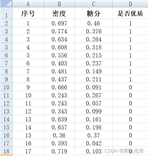
然后就从EXCEL文件里面读取并写入到一个符合LIBSVM格式的文件即可
代码如下:
from libsvm.svm import *
from libsvm.svmutil import *
import openpyxl
import matplotlib as mpl
import matplotlib.pyplot as plt
import numpy as np

def gen_svmfile():
    wb = openpyxl.load_workbook("test/s.xlsx")
    sheet1 = wb['Sheet1']
    with open("test/s_scale", 'w') as f:
        for i in range(1,sheet1.max_row):
            midu = sheet1.cell(i+1,2).value
            tangfen = sheet1.cell(i+1,3).value
            youzhi = sheet1.cell(i+1,4).value
            line = str(youzhi) + " 1:" + str(midu) + " 2:" + str(tangfen)
            print(line)
            f.writelines(line + "\n")
gen_svmfile()
'''
1 1:0.697 2:0.46
1 1:0.774 2:0.376
1 1:0.634 2:0.264
1 1:0.608 2:0.318
1 1:0.556 2:0.215
1 1:0.403 2:0.237
1 1:0.481 2:0.149
1 1:0.437 2:0.211
0 1:0.666 2:0.091
0 1:0.243 2:0.267
0 1:0.245 2:0.057
0 1:0.343 2:0.099
0 1:0.639 2:0.161
0 1:0.657 2:0.198
0 1:0.36 2:0.37
0 1:0.593 2:0.042
0 1:0.719 2:0.103
'''
如果提示相关模块没有安装的情况,类似下面这样安装即可:
pip install openpyxl -i http://pypi.douban.com/simple/ --trusted-host pypi.douban.com6、分类可视化
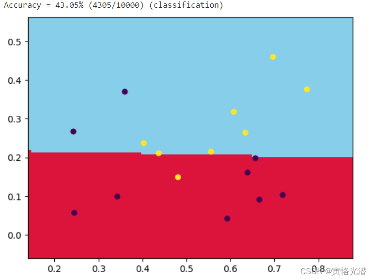
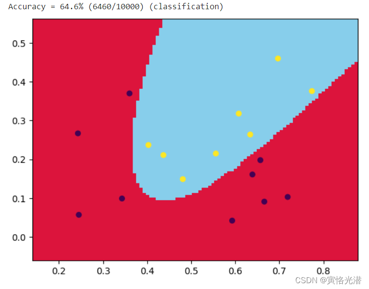
有了数据集之后,我们来看下对水果是否优质进行分类,代码如下:
y, x = svm_read_problem("test/s_scale")
m = svm_train(y, x, '-t 0 -c 100')#线性函数
#m = svm_train(y, x, '-t 2 -c 100')#径向基函数
#m = svm_train(y, x, '-t 2 -c 10000')
x1 = [mapi[1] for mapi in x]
x2 = [mapi[2] for mapi in x]
x = np.c_[x1,x2]

np_x = np.asarray(x)
np_y = np.asarray(y)
N, M = 100, 100

x1_min, x2_min = np_x.min(axis=0)
x1_max, x2_max = np_x.max(axis=0)

x1_min -= 0.1
x2_min -= 0.1
x1_max += 0.1
x2_max += 0.1

t1 = np.linspace(x1_min, x1_max, N)
t2 = np.linspace(x2_min, x2_max, M)
grid_x, grid_y = np.meshgrid(t1,t2)

grid = np.stack([grid_x.flat, grid_y.flat], axis=1)

y_fake = np.zeros((N*M,))
p_label, _, _ = svm_predict(y_fake, grid, m)

cm_light = mpl.colors.ListedColormap(['#DC143C', '#87CEEB'])#颜色更改用来区分下面散点图
plt.pcolormesh(grid_x, grid_y, np.array(p_label).reshape(grid_x.shape), cmap=cm_light)#cm_light直接换成'cool'也可以
#散点图,直观查看制作的那几个点的情况
plt.scatter(x[:,0], x[:,1], s=30, c=y, marker='o')

plt.show()
效果图(-t 0线性函数)svm_train(y, x, '-t 0 -c 100'):
径向基函数(-t 2高斯核函数):svm_train(y, x, '-t 2 -c 100'),效果图如下:
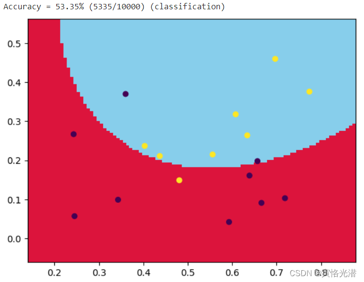
还可以通过提高参数c来提高分类的准确率svm_train(y, x, '-t 2 -c 10000'):
7、np.c_和np.stack
代码当中有两个知识点附带说明下,常用来做数据变换的。
np.c_:拼接的作用,我们分别看下不同维度是如何做拼接的
#一维数组
a1=np.arange(10)
b1=np.arange(10,20)
print(a1,b1)#[0 1 2 3 4 5 6 7 8 9] [10 11 12 13 14 15 16 17 18 19]
print(np.c_[a1,b1])
print(np.c_[a1,b1].shape)#(10, 2)


#二维数组
a2=np.arange(10).reshape(2,5)
b2=np.arange(10,20).reshape(2,5)
print(a2,b2)
'''
[[0 1 2 3 4]
 [5 6 7 8 9]]

[[10 11 12 13 14]
 [15 16 17 18 19]]
'''
print(np.c_[a2,b2].shape)#(2, 10)

#另外一个相反的拼接就是np.r_
print(np.r_[a2,b2].shape)#(4, 5)
我们看形状就很明白了,哪个维度的值不变,哪个维度的值在增加。
np.stack:数组按指定维进行堆叠
所以这里我们只需要关注指定的维度,就能够知道如何堆叠:
#一维数组
a1=np.arange(10)
b1=np.arange(10,20)
print(a1,b1)
print(np.stack([a1,b1]))#默认是axis=0
print(np.stack([a1,b1],axis=0).shape)#(2, 10)
print(np.stack([a1,b1],axis=1).shape)#(10, 2)
#注意观察axis指定位置在第一维和第二维的区别。

#二维数组
a2=np.arange(10).reshape(2,5)
b2=np.arange(10,20).reshape(2,5)
print(a2,b2)
print(np.stack([a2,b2],axis=0).shape)#(2, 2, 5)
print(np.stack([a2,b2],axis=1).shape)#(2, 2, 5)
#这里形状一样,不过内容不一样:
#axis=0的情况
[[[ 0  1  2  3  4]
  [ 5  6  7  8  9]]

 [[10 11 12 13 14]
  [15 16 17 18 19]]]

#axis=1的情况
[[[ 0  1  2  3  4]
  [10 11 12 13 14]]

 [[ 5  6  7  8  9]
[15 16 17 18 19]]]官方站点:https://www.csie.ntu.edu.tw/~cjlin/libsvm/
A Practical Guide to Support Vector Classification(支持向量分类实用指南)
其他版本:https://pypi.org/project/libsvm-official/#files