对于一些流行的机器学习算法,如何设置超参数会极大地影响机器学习算法的性能。
一种简单暴力的方法是遍历超参数空间的不同组合并选择最佳配置。 这称为网格搜索策略 (Grid Search)。 但是这种方法收敛速度非常慢。
更好的方法是使用某种优化方法来优化我们的优化算法。 Optuna 和 Hyperopt 等工具在此发挥作用。
在下文中,我们将使用 Optuna 作为示例,并将其应用于随机 森林 分类器。
1. 导入库并获取新闻组数据
import numpy as np
import os
from sklearn.datasets import fetch_20newsgroups
from sklearn.model_selection import cross_val_score
from sklearn.metrics import f1_score
from sklearn.feature_extraction.text import TfidfVectorizer
from sklearn.pipeline import Pipeline
import joblib
from lightgbm import LGBMClassifier
from sklearn.ensemble import RandomForestClassifier

import optuna

data = fetch_20newsgroups()

X = data['data'][:5000]
y = data['target'][:5000]
2. 使用 TfidfVectorizer 和 RandomForestClassifier 定义机器学习Pipeline
model = Pipeline([
    ('tfidf', TfidfVectorizer(stop_words='english')),
    ('rf', RandomForestClassifier())
])
3. 定义超参数空间和 Optuna 目标函数以进行优化
def objective(trial):

    joblib.dump(study, 'study.pkl')

    tfidf__analyzer = trial.suggest_categorical('tfidf__analyzer', ['word', 'char', 'char_wb'])
    tfidf__lowercase = trial.suggest_categorical('tfidf__lowercase', [False, True])
    tfidf__max_features = trial.suggest_int('tfidf__max_features', 500, 10_000)
    rf__n_estimators = trial.suggest_int('rf__num_estimators', 300, 500)
    rf__max_depth = trial.suggest_int('rf__max_depth', 5, 15)
    rf__min_samples_split = trial.suggest_int('rf__min_samples_split', 10, 30)


    params = {
        'tfidf__analyzer': tfidf__analyzer,
        'tfidf__lowercase': tfidf__lowercase,
        'tfidf__max_features': tfidf__max_features,
        'rf__n_estimators': rf__n_estimators,
        'rf__max_depth': rf__max_depth,
        'rf__min_samples_split': rf__min_samples_split,

    }

    model.set_params(**params)

    return  -np.mean(cross_val_score(model, X, y, cv=3, n_jobs=-1,scoring='neg_log_loss'))
请注意,默认情况下,Optuna 尝试最小化目标函数,因为我们使用原始机器学习算法的对数损失函数来最大化随机森林分类器,所以我们在交叉验证分数前面添加了另一个负号。
4. 运行 Optuna 试验以找到最佳的超参数配置
# by default, the direction is to minimizae, but can set it to maximize too
#study = optuna.create_study(direction='minimize')
study = optuna.create_study()


#study.optimize(objective, timeout=3600)
study.optimize(objective, n_trials=20)


# to record the value for the last time
joblib.dump(study, 'study.pkl')
请注意,我们将超参数优化过程保存到本地 pickle 文件中,这意味着我们可以通过打开另一个笔记本来监控中途或结束时的过程。
5. 优化过程和结果可视化
%matplotlib inline
import joblib
import pandas as pd
import numpy as np
import matplotlib.pyplot as plt
import seaborn as sns
import optuna
data = joblib.load('study.pkl')
df = data.trials_dataframe()
df.dropna(inplace=True)
df.reset_index(inplace=True)
df['time'] = (df.datetime_complete - df.datetime_start).dt.total_seconds()
df = df[df.time>=0]
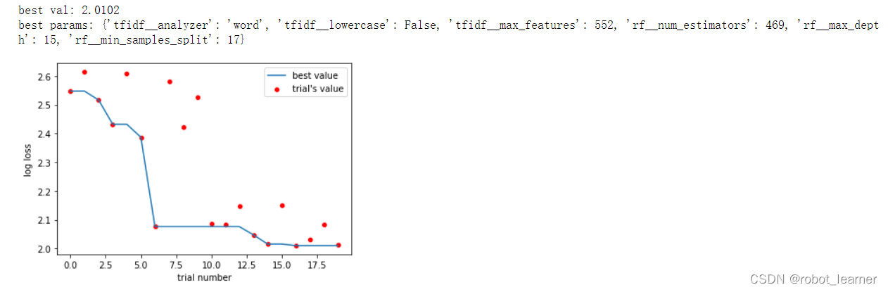
print('best val:', round(df.value.min(),4))
print('best params:', data.best_params)
a = sns.lineplot(x=df.index, y=df.value.cummin())
a.set_xlabel('trial number')
sns.scatterplot(x=df.index, y=df.value, color='red')
a.set_ylabel('log loss')
a.legend(['best value', "trial's value"]);
6. 代码notebook下载
下载全部代码,请点击英文link的最后
code link