神经网络万能近似定理探索与实验
今天,我们来做神经网络万能近似定理的探索与实验。关于万能近似定理呢,就是说,对这个神经元的输出进行非线性激活函数处理,单层的神经网络就可以拟合任何一个函数。
下面先看我们搭建的第一个网络结构图:
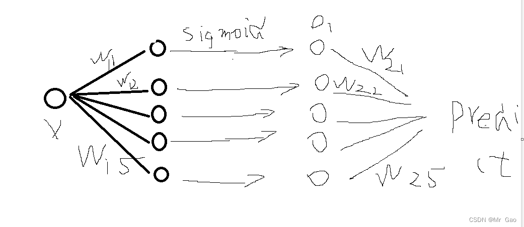
画的可能有点丑,就是搭建了一个隐藏层,使用sigmoid进行处理,最后加一个全连接层输出结果作为预测结果。
在实验中,我们使用的拟合函数是y=x+x^2+3
#coding=gbk

import torch
from torch.autograd import Variable
from torch.utils import data
import matplotlib.pyplot as plt

neuron_num=10
batch=32
sample_num=300
learn_rating=0.001
epoch=1000


x_data=torch.linspace(0,172,sample_num)
#print(x_data)

torch.manual_seed(10)

def function(x):
  return x*2+x**2+3
y_real=function(x_data)
#print(y_real)


def sampling(sample_num):

    #print(data_size)
    index_sequense=torch.randperm(sample_num)
    return index_sequense

w=torch.rand(neuron_num)
b=torch.randn(neuron_num)
w2=torch.randn(neuron_num)
b2=torch.randn(1)
def activation_function(x):
    return 1/(1+torch.sigmoid(-x))


def hidden_layer(w,b,x):
    return activation_function(w*x+b)

def  fully_connected_layer(w2,b2,x):
    return torch.dot(w2,x)+b2

def net(w,b,w2,b2,x):
    #print("w",w)
    #print("b",b)
    o1=hidden_layer(w,b,x)
    #print("o1",o1)
    #print("w2",w2)
    #print("b2",b2)
    o2=fully_connected_layer(w2,b2,o1)
 #   print("o2",o2)

    return o2

def get_grad(w,b,w2,b2,x,y_predict,y_real):


    o2=hidden_layer(w,b,x)

    l_of_w2=-(y_real-y_predict)*o2
    l_of_b2=-(y_real-y_predict)
    l_of_w=-(y_real-y_predict)*torch.dot(w2,o2*(1-o2))*x
    l_of_b=-(y_real-y_predict)*torch.dot(w2,o2*(1-o2))
    #print("grad")
    #print(l_of_w)
    #print(l_of_w2)
    #print(l_of_b)
    #print(l_of_b2)
    return l_of_w2,l_of_b2,l_of_w,l_of_b

def loss_function(y_predict,y_real):
    #print(y_predict,y_real)
    return torch.pow(y_predict-y_real,2)
loss_list=[]


def train():
    global w,w2,b,b2
    index=0
    for i in range(epoch):

        index_sequense=sampling(sample_num)

        W_g=torch.zeros(neuron_num)
        b_g=torch.zeros(neuron_num)
        W2_g=torch.zeros(neuron_num)
        b2_g=torch.zeros(1)
        loss=torch.tensor([0.0])

        for k in range(batch):
              try:
                   # print("x",x_data[index],index)
                   # print("w",w)
                        y_predict=net(w,b,w2,b2,x_data[index_sequense[index]])
                        #print("y_predict",y_predict)
                        #print("x:",x_data[index_sequense[index]])
                        #print("yreal:",y_real[index_sequense[index]])
                        get_grad(w,b,w2,b2,x_data[index_sequense[index]],y_predict,y_real[index_sequense[index]])

                        l_of_w2,l_of_b2,l_of_w,l_of_b= get_grad(w,b,w2,b2,x_data[index_sequense[index]],y_predict,y_real[index_sequense[index]])
                        W_g=W_g+l_of_w
                        b_g=b_g+l_of_b
                        b2_g=b2_g+l_of_b2
                        W2_g=W2_g+l_of_w2
                        loss=loss+loss_function(y_predict,y_real[index_sequense[index]])
                        index=index+1


              except:
                        index=0
                        index_sequense=sampling(sample_num)
        print("****************************loss is :",loss/batch)
        loss_list.append(loss/batch)

        W_g=W_g/batch
        b_g=b_g/batch
        b2_g=b2_g/batch
        W2_g=W2_g/batch
        w=w-learn_rating*W_g
        b=b-learn_rating*b_g
        w2=w2-learn_rating*W2_g
        b2=b2-learn_rating*b2_g
        #print(W2_g/batch)
        #print('w2',w2)
        #print(W_g/batch)
        #print('w1',w)


train()

y_predict=[]
for i in range(sample_num):

  y_predict.append(net(w,b,w2,b2,x_data[i]))

epoch_list=list(range(epoch))
plt.plot(epoch_list,loss_list,label='SGD')
plt.title("loss")
plt.legend()

plt.show()

plt.plot(x_data,y_real,label='real')
plt.plot(x_data,y_predict,label='predict')
plt.title(" Universal Theorem of Neural Networks")
plt.legend()
plt.show()
print(w,b,w2,b2)
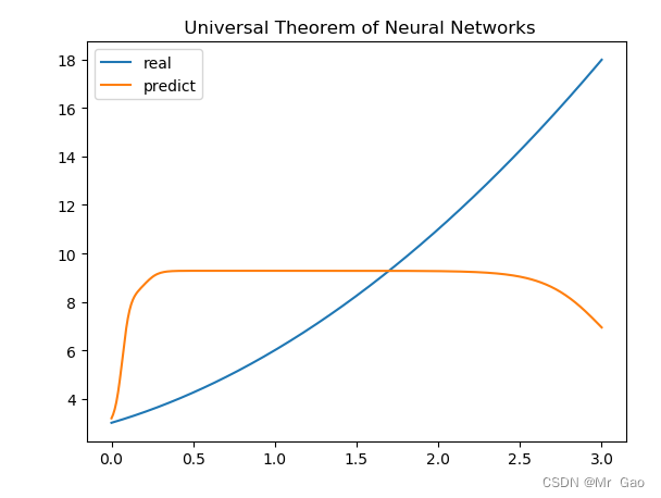
跑出的实验结果如下:
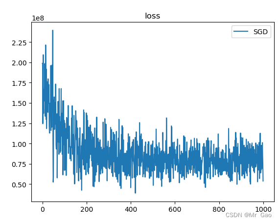
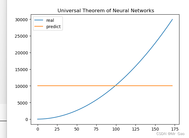
可以看到模型确实是由一定效果的,但是后面为什么跑出来的结果是一个直线呢,因为博主在推导的时候发现,w2i,i=1,2,的权重迭代时等量的,所以,才会出现这样的情况,因为神经元参数等量更新了,而且时同时更新,而且经过sigmoid转化,数值变为了1,才会发生这样的拟合情况。同时因为博主数据集真是的拟合值太大了,才会出现这样的问题
现在我们调整一下数据集
修改上述如下代码:
neuron_num=5
batch=32
sample_num=300
learn_rating=0.001
epoch=100


x_data=torch.linspace(0,3,sample_num)
#print(x_data)

torch.manual_seed(10)

def function(x):
  return x*2+x**2+3
y_real=function(x_data)
#print(y_real)


wz=torch.rand(neuron_num)
#print(wz)
w=torch.normal(0,10,size=(neuron_num,))
b=torch.normal(0,10,size=(neuron_num,))
w2=torch.normal(0,10,size=(neuron_num,))
b2=torch.normal(0,10,size=(1,))
#print(w,b)
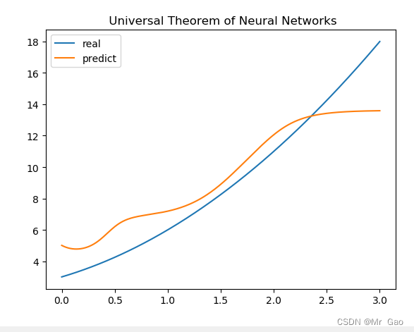
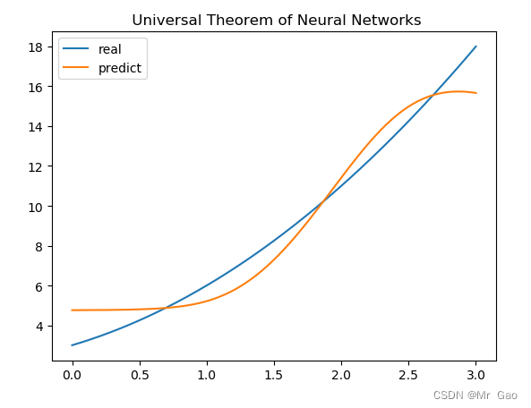
会跑出下面一个结果:
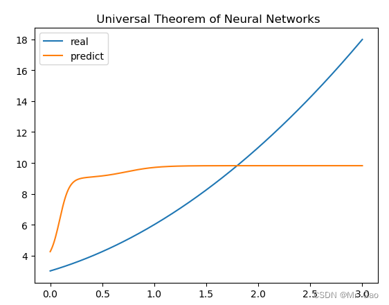
看起来是不是好了一点,现在我们增加训练轮次,来看一下:
neuron_num=5
batch=32
sample_num=300
learn_rating=0.001
epoch=1000
跑出的结果:
增加神经元数量:
neuron_num=10
batch=32
sample_num=300
learn_rating=0.001
epoch=1000
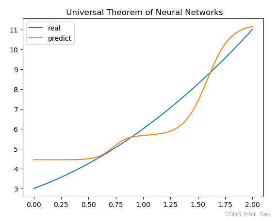
这个时候奇迹发生了:
loss结果:
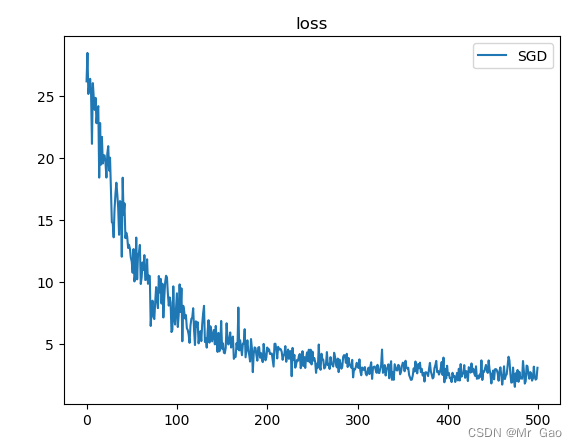
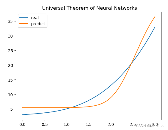
拟合结果
我们继续增加神经元个数,增加到20:
neuron_num=20
batch=32
sample_num=300
learn_rating=0.01
epoch=1000
其实博主后来发现了,学习率也很重要,也不是说神经元越多越好,学习率也是很重要的一方面。
还有一百个神经元的:
neuron_num=100
batch=32
sample_num=300
learn_rating=0.01
epoch=1000
结果呢,可能还要好一点,sigmoid函数其实还好,还是很不错的,如果随着我们神经元的增多,确实效果会越来越好。
后面博主将函数改的更复杂了一些,跑出来结果也不错:
neuron_num=1000
batch=32
sample_num=300
learn_rating=0.001
epoch=3000


#print(x_data)


torch.manual_seed(10)

x_data=torch.linspace(0,3,sample_num)
def function(x):
  return x+x**3+3
y_real=function(x_data)
#print(y_real)
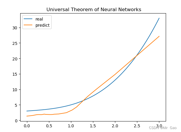
结果如下:
当然,越复杂的函数可能就需要越多的神经元,同时神经元初始化的数据也很重要,是否能很好的学习我们设定的函数并不是那么容易需要很多因素的功能作用,都需要我们去调整。
下面博主有做了relu激活函数的拟合代码,代码如下:
#coding=gbk

import torch
from torch.autograd import Variable
from torch.utils import data
import matplotlib.pyplot as plt

neuron_num=50

batch=32
sample_num=300
learn_rating=0.001
epoch=1000


#print(x_data)


torch.manual_seed(10)

x_data=torch.linspace(0,3,sample_num)
def function(x):
  return x+x**3+3
y_real=function(x_data)
#print(y_real)


wz=torch.rand(neuron_num)
#print(wz)
w=torch.normal(0,1,size=(neuron_num,))
b=torch.normal(0,1,size=(neuron_num,))
w2=torch.normal(0,1,size=(neuron_num,))
b2=torch.normal(0,1,size=(1,))
#print(w,b)


def sampling(sample_num):

    #print(data_size)
    index_sequense=torch.randperm(sample_num)
    return index_sequense
def activation_function(x):
    return 1/(1+torch.sigmoid(-x))


def activation_function2(x):

   # print(x.size())
    a=torch.rand(x.size())
    for i in range(x.size(0)):
        if x[i]<=0:
            a[i]=0.0
        else:
            a[i]=x[i]
    return a


def hidden_layer(w,b,x):
   # print("x:",x)
    return activation_function2(w*x+b)

def  fully_connected_layer(w2,b2,x):
    return torch.dot(w2,x)+b2

def net(w,b,w2,b2,x):
    #print("w",w)
    #print("b",b)
    o1=hidden_layer(w,b,x)
    #print("o1",o1)
    #print("w2",w2)
    #print("b2",b2)
    o2=fully_connected_layer(w2,b2,o1)
 #   print("o2",o2)

    return o2

def get_grad(w,b,w2,b2,x,y_predict,y_real):


    o2=hidden_layer(w,b,x)

    l_of_w2=-(y_real-y_predict)*o2
    l_of_b2=-(y_real-y_predict)

    a=torch.rand(o2.size())
    for i in range(o2.size(0)):
        if o2[i]<=0:
            a[i]=0.0
        else:
            a[i]=1
    l_of_w=-(y_real-y_predict)*torch.dot(w2,a)*x
    l_of_b=-(y_real-y_predict)*torch.dot(w2,a)
    #print("grad")
    #print(l_of_w)
    #print(l_of_w2)
    #print(l_of_b)
    #print(l_of_b2)
    return l_of_w2,l_of_b2,l_of_w,l_of_b

def loss_function(y_predict,y_real):
    #print(y_predict,y_real)
    return torch.pow(y_predict-y_real,2)
loss_list=[]


def train():
    global w,w2,b,b2
    index=0
    for i in range(epoch):

        index_sequense=sampling(sample_num)

        W_g=torch.zeros(neuron_num)
        b_g=torch.zeros(neuron_num)
        W2_g=torch.zeros(neuron_num)
        b2_g=torch.zeros(1)
        loss=torch.tensor([0.0])

        for k in range(batch):
              try:
                   # print("x",x_data[index],index)
                   # print("w",w)
                        y_predict=net(w,b,w2,b2,x_data[index_sequense[index]])
                        #print("y_predict",y_predict)
                        #print("x:",x_data[index_sequense[index]])
                        #print("yreal:",y_real[index_sequense[index]])
                        get_grad(w,b,w2,b2,x_data[index_sequense[index]],y_predict,y_real[index_sequense[index]])

                        l_of_w2,l_of_b2,l_of_w,l_of_b= get_grad(w,b,w2,b2,x_data[index_sequense[index]],y_predict,y_real[index_sequense[index]])
                        W_g=W_g+l_of_w
                        b_g=b_g+l_of_b
                        b2_g=b2_g+l_of_b2
                        W2_g=W2_g+l_of_w2
                        loss=loss+loss_function(y_predict,y_real[index_sequense[index]])
                        index=index+1


              except:
                        index=0
                        index_sequense=sampling(sample_num)
        print("****************************loss is :",loss/batch)
        loss_list.append(loss/batch)

        W_g=W_g/batch
        b_g=b_g/batch
        b2_g=b2_g/batch
        W2_g=W2_g/batch
        w=w-learn_rating*W_g
        b=b-learn_rating*b_g
        w2=w2-learn_rating*W2_g
        b2=b2-learn_rating*b2_g
        #print(W2_g/batch)
        #print('w2',w2)
        #print(W_g/batch)
        #print('w1',w)


#print(x_data.size())
y_predict=net(w,b,w2,b2,x_data[0])

train()

y_predict=[]
for i in range(sample_num):

  y_predict.append(net(w,b,w2,b2,x_data[i]))

epoch_list=list(range(epoch))
plt.plot(epoch_list,loss_list,label='SGD')
plt.title("loss")
plt.legend()

plt.show()

plt.plot(x_data,y_real,label='real')
plt.plot(x_data,y_predict,label='predict')
plt.title(" Universal Theorem of Neural Networks")
plt.legend()
plt.show()
print(w,b,w2,b2)
下面时拟合结果:
个人觉得relu函数的拟合性要比sigmoid函数强一点。好的,本次实验到此位置,感兴趣的同学可以多学习一下哈。