文章目录
前言
上次学习笔记介绍了决策树算法,它是机器学习中简单而高效的一个模型,即便如此,决策树毕竟势单力薄,也有很多问题无法解决,但如果我们引入多棵树那情况就有所改善。如果说树作为自然界的个体,那么森林就是群体,个体的集合。随机森林模型,从字面上说就是用随机的方式建立一个森林,森林里面有很多的决策树组成,随机森林的每一棵决策树之间是没有关联的,增强了树个体的多样性和整个森林竞争能力。
一、集成学习简介
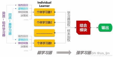
集成算法主要会构建多个学习器,通过一定策略结合来完成学习任务。正所谓三个臭皮匠顶一个诸葛亮,当弱学习器被正确组合时,我们能得到更精确、鲁棒性更好的学习器。由于个体学习器在准确性和多样性存在冲突,追求多样性势必要牺牲准确性。这就需要将这些“好而不同”的个体学习器结合起来。这就好像在一片森林中,不同的树的生存能力不同,将它们结合起来就会得到更茂盛的丛林。
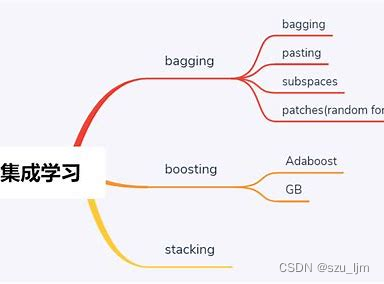
按照个体学习器之间的关系,集成算法分为Bagging、Boosting、Stacking三大类。
基于Bagging算法
Bagging算法(装袋法)是bootstrap aggregating的缩写,它主要对样本训练集合进行随机化抽样,通过反复的抽样训练新的模型,最终在这些模型的基础上取平均。
基于Boosting算法
提升算法(Boosting)是常用的有效的统计学习算法,属于迭代算法,它通过不断地使用一个弱学习器弥补前一个弱学习器的“不足”的过程,来串行地构造一个较强的学习器,这个强学习器能够使目标函数值足够小。
基于Stacking算法
在模型预测得到的结果上,再训练一个模型,就仿佛是在原有的模型上再「堆叠」(Stacking)一个模型。Stacking 能够把各个模型在提取特征较好的部分给抓取出来,同时舍弃它们各自表现不好的部分,这就能够有效地优化预测结果、提高最终预测的分数了。
二、集成学习的数学原理
1. 随机森林算法
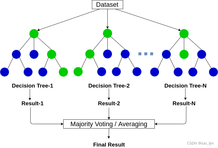
Bagging的核心思想是,假设有一个大小为 N 的训练数据集,每次从该数据集中有放回的取出样本数量为 K K K 的子数据集,一共选 M M M 次,根据这 M M M 个子数据集,训练学习出 M M M 个模型。当要预测的时候,使用这 M M M 个模型进行预测,再通过取平均值或者多数分类的方式,得到最后的预测结果,我们用 f ( x ) f(x) f(x) 来表达最终的分类器
f ( x ) = 1 m ∑ i = 1 m f i ( x ) f(x) = \frac{1}{m} \sum_{i=1}^{m} f_{i}(x) f(x)=m1i=1∑mfi(x)
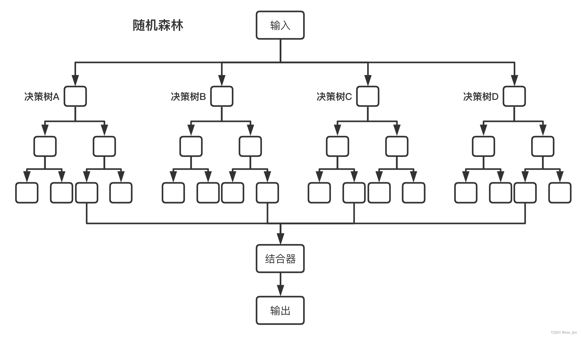
随机森林遵循Bagging的核心思想,假设有一个大小为 N N N 的训练数据集, 该数据集有 M M M 个特征,, 首先通过有放回的随机抽样的方法抽取 k k k 个样本作为单棵决策树模型的样本数据, 并同时随机选择 n n n 个特征作为该决策树的节点属性,然后按照决策树的训练方法并行生成 m m m 棵树,最后对 n n n 棵决策树的分类效果取平均
2. Adaboost算法
Boosting算法的核心思想是,我们先训练一个弱学习器,下一轮迭代产生的分类器是在上一轮的弱学习器基础上训练得来的,即下一轮的弱学习器会基于上一轮分类产生的误差来进行新的学习,尽量降低该轮学习器分类产生的误差,最后将前一个弱学习器的结果和当前弱学习器按一定的权重来更新当前的强学习器的模型。我们用 F ( x ) F(x) F(x) 来表达学习器,我们希望是新一轮学习器 h ( x ) h(x) h(x) 和旧学习器的组合能使损失最低
F m ( x ) = F m − 1 ( x ) + a r g m i n h ∈ H ∑ i = 1 n L o s s ( y i , F m − 1 ( x i ) + h ( x i ) ) F_{m}(x) = F_{m-1} (x) + argmin_{h \in H} \sum_{i=1}^{n} Loss(y_{i}, F_{m-1}(x_{i})+h(x_{i})) Fm(x)=Fm−1(x)+argminh∈Hi=1∑nLoss(yi,Fm−1(xi)+h(xi))
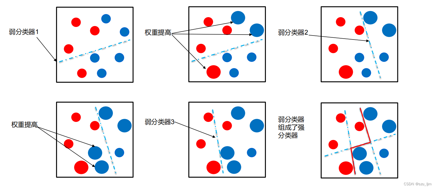
Adaboost算法就是基于boosting策略,首先初始化训练样本的权值分布,每个样本具有相同权重;接着训练弱分类器,如果样本分类正确,则在构造下一个训练集中,它的权值就会被降低,样本分类错误就会被提高,就像你考试做错题,你就会对错题格外关注不断重做,而对待熟悉做对的题不用花过多时间。用更新过的样本集去训练下一个分类器;各个弱分类器的训练过程结束后,加大分类误差率小的弱分类器的权重,降低分类误差率大的弱分类器的权重,将所有弱分类组合成强分类器。
3. GBDT算法
Gradient Boosting策略是基于Boosting策略进行的,它的核心思想是串行地生成多个弱学习器,每个弱学习器的目标是拟合先前累加模型的损失函数的负梯度, 使加上该弱学习器后的累积模型损失往负梯度的方向减少。如果第 m m m 轮弱学习器拟合损失函数关于累积模型的负梯度,则加上该弱学习器之后累积模型的 L o s s Loss Loss 会最小,分类效果越好。
∇ g m = ∂ L o s s ( y , F m − 1 ( x ) ) ∂ F m − 1 ( x ) \nabla g_{m} = \frac{ \partial Loss(y,F_{m-1}(x)) }{ \partial F_{m-1}(x) } ∇gm=∂Fm−1(x)∂Loss(y,Fm−1(x))
GBDT 算法基于Gradient Boosting策略,每个弱学习器都是 CART 回归树,在回归问题中,损失函数采用均方损失函数:
L o s s ( y , F m − 1 ( x ) ) = ( y − F m − 1 ( x ) ) 2 Loss(y,F_{m-1}(x)) =(y-F_{m-1}(x))^{2} Loss(y,Fm−1(x))=(y−Fm−1(x))2
每棵CART决策树会朝着拟合前一轮累积模型产生的损失函数梯度的目标去生成,在这一轮累积模型中使损失不断降低,通过这样不断迭代生成强学习器,其实这个过程是利用梯度下降的思想来达到更好的分类效果
三、Python实现集成学习算法
1. 随机森林算法
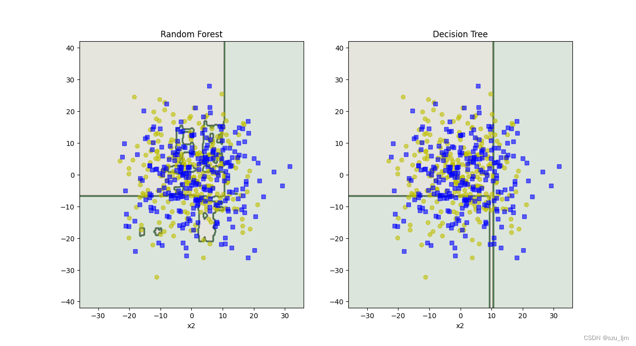
Python实现随机森林算法的思路也和前面一样,先导入常用的包和月亮数据集,接着将随机森林和决策树实例化进行对比,分别训练决策树和随机森林并进行分类,然后用matplotlib绘制棋盘和决策边界,最后展示一下
import numpy as np
import matplotlib.pyplot as plt
from sklearn.ensemble import RandomForestClassifier
from sklearn.tree import DecisionTreeClassifier
from sklearn.model_selection import train_test_split
from sklearn.datasets import make_moons
from matplotlib.colors import ListedColormap

x, y = make_moons(n_samples=500, noise=10, random_state=56)
x_train, x_test, y_train, y_test = train_test_split(x, y, random_state=56)
RF_clf = RandomForestClassifier(n_estimators=500, max_depth=3, criterion='gini', min_samples_leaf=8, bootstrap=True, n_jobs=-1, random_state=56)
RF_clf.fit(x_train, y_train)
y_RF_pred = RF_clf.predict(x_test)
tree_clf = DecisionTreeClassifier(random_state=56, max_depth=3, min_samples_leaf=8, criterion='gini')
tree_clf.fit(x_train, y_train)
y_tree_pred = tree_clf.predict(x_test)


def plot_decision_boundary(clf, x, y, alpha=0.5):
    axes = [-36, 36, -42, 42]
    x1s = np.linspace(axes[0], axes[1], 300)
    x2s = np.linspace(axes[2], axes[3], 300)
    x1, x2 = np.meshgrid(x1s, x2s)
    x_new = np.c_[x1.ravel(), x2.ravel()]
    y_pred = clf.predict(x_new).reshape(x1.shape)
    custom_cmap2 = ListedColormap(['#7d7d58', '#4c4c7f', '#507d50'])
    plt.contour(x1, x2, y_pred, cmap=custom_cmap2, alpha=0.8)
    plt.contourf(x1, x2, y_pred, cmap=custom_cmap2, alpha=0.2)
    plt.plot(x[:, 0][y == 0], x[:, 1][y == 0], 'yo', alpha=0.6)
    plt.plot(x[:, 0][y == 1], x[:, 1][y == 1], 'bs', alpha=0.6)
    plt.xlabel('x1')
    plt.xlabel('x2')

plt.figure(figsize=(12,8))
plt.subplot(121)
plot_decision_boundary(RF_clf, x, y)
plt.title('Random Forest')
plt.subplot(122)
plot_decision_boundary(tree_clf, x, y)
plt.title('Decision Tree')
plt.show()
2. Adaboost算法
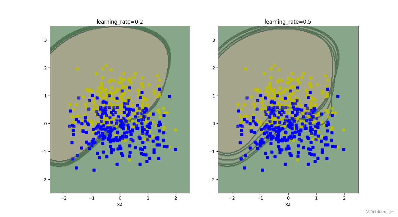
Python实现Adaboost算法的思路也和前面一样,先导入常用的包和月亮数据集,接着将支持向量机SVM作为单个学习器进行实例化,迭代式训练SVM进行分类并对不同效果的SVM分类器进行加权,针对SVM学习器学的不好的地方加大它的学习率,然后用matplotlib绘制棋盘和决策边界,最后展示一下
import numpy as np
import matplotlib.pyplot as plt
from sklearn.model_selection import train_test_split
from sklearn.svm import SVC
from sklearn.datasets import make_moons
from matplotlib.colors import ListedColormap

x, y = make_moons(n_samples=500, noise=0.5, random_state=56)
x_train, x_test, y_train, y_test = train_test_split(x, y, random_state=56)


def plot_decision_boundary(clf, x, y):
    axes = [-2.5, 2.5, -2.5, 3.5]
    x1s = np.linspace(axes[0], axes[1], 200)
    x2s = np.linspace(axes[2], axes[3], 200)
    x1, x2 = np.meshgrid(x1s, x2s)
    x_new = np.c_[x1.ravel(), x2.ravel()]
    y_pred = clf.predict(x_new).reshape(x1.shape)
    custom_cmap2 = ListedColormap(['#7d7d58', '#4c4c7f', '#507d50'])
    plt.contour(x1, x2, y_pred, cmap=custom_cmap2, alpha=0.8)
    plt.contourf(x1, x2, y_pred, cmap=custom_cmap2, alpha=0.2)
    plt.plot(x[:, 0][y == 0], x[:, 1][y == 0], 'yo', alpha=0.6)
    plt.plot(x[:, 0][y == 0], x[:, 1][y == 1], 'bs', alpha=0.6)
    plt.xlabel('x1')
    plt.xlabel('x2')

m = len(x_train)

plt.figure(figsize=(12, 8))

for subplot, learning_rate in ((121, 0.2), (122, 0.5)):
    sample_weights = np.ones(m)
    plt.subplot(subplot)
    for i in range(5):
        svm_clf = SVC(kernel='rbf', C=0.05, random_state=56)
        svm_clf.fit(x_train, y_train, sample_weight=sample_weights)
        y_pred = svm_clf.predict(x_train)
        sample_weights[y_pred != y_train] *= (1 + learning_rate)
        plot_decision_boundary(svm_clf, x, y)
        plt.title('learning_rate={}'.format(learning_rate))


plt.show()
3. GBDT算法
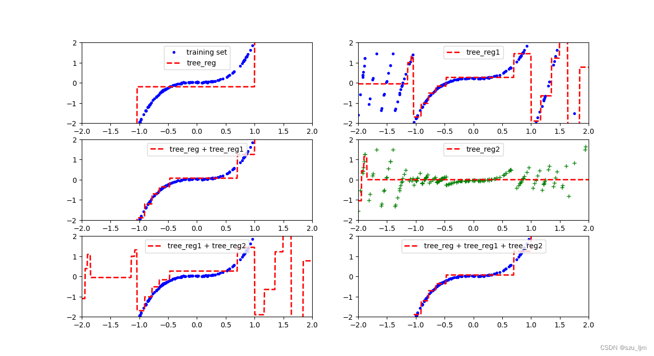
Python实现GBDT算法的思路也和前面一样,先导入常用的包并自己生成一个非线性函数进行拟合,接着将决策树作为单个学习器进行实例化,这里的决策树主要起到回归拟合的作用,迭代式训练决策树进行回归,让下一轮决策树对上一轮产生的损失进行学习拟合,然后用matplotlib绘制棋盘和决策边界,最后展示一下
import numpy as np
import matplotlib.pyplot as plt
from sklearn.tree import DecisionTreeRegressor

np.random.seed(36)
x = np.random.randn(200, 1) - 0.3
y0 = 2*x[:, 0]**3 + 0.05*np.random.rand(200)


def plot_predictions(regs, x, y, axes, label=None, data_label=None, style="r--", data_style="b.",):
    x1 = np.linspace(axes[0], axes[1], 600)
    y_pred = np.sum(reg.predict(x1.reshape(-1, 1)) for reg in regs)
    plt.plot(x[:, 0], y, data_style, label=data_label)
    plt.plot(x1, y_pred, style, label=label, linewidth=2)
    if data_label or label:
        plt.legend(loc="upper center", fontsize=10)
    plt.axis(axes)


tree_reg = DecisionTreeRegressor(max_depth=4)
tree_reg.fit(x, y0)

y1 = y0 - tree_reg.predict(x)
tree_reg1 = DecisionTreeRegressor(max_depth=4)
tree_reg1.fit(x, y1)

y2 = y1 - tree_reg1.predict(x)
tree_reg2 = DecisionTreeRegressor(max_depth=4)
tree_reg2.fit(x, y2)

plt.figure(figsize=(12, 8))

plt.subplot(321)
plot_predictions([tree_reg], x, y0, axes=[-2, 2, -2, 2], label='tree_reg', data_label='training set')
plt.subplot(322)
plot_predictions([tree_reg1], x, y1, axes=[-2, 2, -2, 2], label='tree_reg1')
plt.subplot(323)
plot_predictions([tree_reg, tree_reg1], x, y0, axes=[-2, 2, -2, 2], label='tree_reg + tree_reg1')
plt.subplot(324)
plot_predictions([tree_reg2], x, y2, axes=[-2, 2, -2, 2], label='tree_reg2', data_style="g+")
plt.subplot(325)
plot_predictions([tree_reg1, tree_reg2], x, y0, axes=[-2, 2, -2, 2], label='tree_reg1 + tree_reg2')
plt.subplot(326)
plot_predictions([tree_reg, tree_reg1, tree_reg2], x, y0, axes=[-2, 2, -2, 2], label='tree_reg + tree_reg1 + tree_reg2')
plt.show()
总结
以上就是机器学习集成算法的学习笔记,本片笔记简单记录了常见的集成算法和Python实现的思路。集思广益是流传千古的智慧,集成算法将不同的学习器结合起来从而达到更加强大的学习效果,在达成不错效果的同时也具有极强的模型泛化能力和高度的可解释性。在深度神经网络称霸的今天,集成学习仍然有其存在和发展的不可替代性。