说明
HBV模型包括一系列自由参数,其值可以通过率定得到。同时也包括一些描述流域和气候特征的参数,它们的值在模型率定是假定不变。子流域的划分使得在一个子流域中可能有很多参数值。虽然在大多数应用中,各子流域之间参数值只有很小的变化,但仍应慎重选取这些参数。
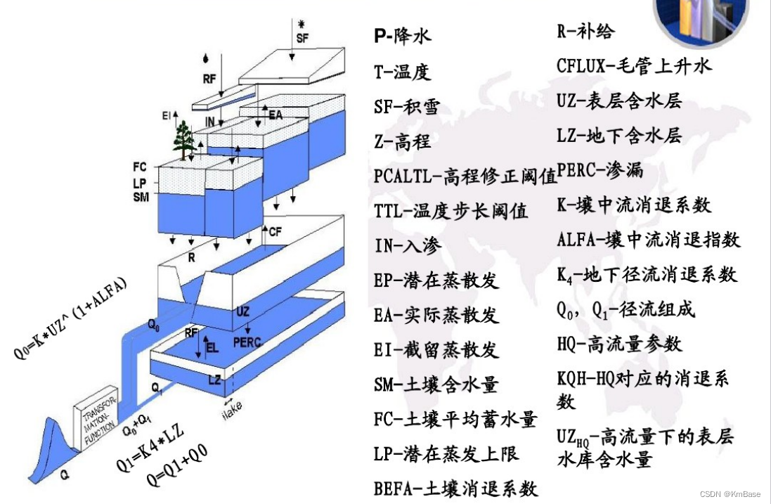
HBV模型主要包括三个子程序:积雪及融雪模块在上层、土壤含水量计算在中层、响应路线在底层。
可以根据流域水系拓朴结构,分别模拟各子流域的径流过程,确定各子流域产流到达总流域出口所流经的子流域,计算各子流域径流到达总流域的出口时间,最后根据汇流时间叠加总流域产流量,形成流域总出口的径流过程。
以下代码,仅包含产流部分,请酌情参考~
源代码
输入数据:逐日降水、逐日气温
输出数据:逐日产流
import numpy as np
import matplotlib.pyplot as plt
"""
Citation:
AghaKouchak A., Habib E., 2010, Application of a Conceptual Hydrologic
Model in Teaching Hydrologic Processes, International Journal of Engineering Education, 26(4), 963-973.
AghaKouchak A., Nakhjiri N., and Habib E., 2012, An educational model for ensemble streamflow
simulation and uncertainty analysis, Hydrology and Earth System Sciences Discussions, 9, 7297-7315, doi:10.5194/hessd-9-7297-2012.
"""
def nse_cost(p):
"""
Purpose:
"""
# Call HBV model
q_sim = hbv_main(len(temp), p, temp, precip, dpem)
# Calculate Nash-Sutcliffe Efficiency
nse = 1.0 - (np.sum((q_obs - q_sim) ** 2.)) / (np.sum((q_obs - np.mean(q_obs)) ** 2.))
nse = 1.0 - nse
return nse
def hbv_main(n_days, params, air_temp, prec, dpem):
Tsnow_thresh = 0.0
ca = 410.
# Initialize arrays for the simiulation
snow = np.zeros(air_temp.size) #
liq_water = np.zeros(air_temp.size) #
pe = np.zeros(air_temp.size) #
soil = np.zeros(air_temp.size) #
ea = np.zeros(air_temp.size) #
dq = np.zeros(air_temp.size) #
s1 = np.zeros(air_temp.size) #
s2 = np.zeros(air_temp.size) #
q = np.zeros(air_temp.size) #
qm = np.zeros(air_temp.size) #
# Set parameters
d = params[0] #
fc = params[1] #
beta = params[2] #
c = params[3] #
k0 = params[4] #
l = params[5] #
k1 = params[6] #
k2 = params[7] #
kp = params[8] #
pwp = params[9] #
for i_day in range(1, n_days):
# print i_day
if air_temp[i_day] < Tsnow_thresh:
# Precip adds to the snow pack
snow[i_day] = snow[i_day - 1] + prec[i_day]
# Too cold, no liquid water
liq_water[i_day] = 0.0
# Adjust potential ET base on difference between mean daily temp
# and long-term mean monthly temp
pe[i_day] = (1. + c * (air_temp[i_day] - monthly[month[i_day]])) * dpem[month[i_day]]
# Check soil moisture and calculate actual evapotranspiration
if soil[i_day - 1] > pwp:
ea[i_day] = pe[i_day]
else:
# Reduced ET_actual by fraction of permanent wilting point
ea[i_day] = pe[i_day] * (soil[i_day - 1] / pwp)
# See comments below
dq[i_day] = liq_water[i_day] * (soil[i_day - 1] / fc) ** beta
soil[i_day] = soil[i_day - 1] + liq_water[i_day] - dq[i_day] - ea[i_day]
s1[i_day] = s1[i_day - 1] + dq[i_day] - max(0, s1[i_day - 1] - l) * k0 - (s1[i_day] * k1) - (
s1[i_day - 1] * kp)
s2[i_day] = s2[i_day - 1] + s1[i_day - 1] * kp - s2[i_day] * k2
q[i_day] = max(0, s1[i_day] - l) * k0 + (s1[i_day] * k1) + (s2[i_day] * k2)
qm[i_day] = (q[i_day] * ca * 1000.) / (24. * 3600.)
else:
# Air temp over threshold: precip falls as rain
snow[i_day] = max(snow[i_day - 1] - d * air_temp[i_day] - Tsnow_thresh, 0.)
liq_water[i_day] = prec[i_day] + min(snow[i_day], d * air_temp[i_day] - Tsnow_thresh, 0.)
# PET adjustment
pe[i_day] = (1. + c * (air_temp[i_day] - monthly[month[i_day]])) * dpem[month[i_day]]
if soil[i_day - 1] > pwp:
ea[i_day] = pe[i_day]
else:
ea[i_day] = pe[i_day] * soil[i_day] / pwp
# Effective precip (portion that contributes to runoff)
dq[i_day] = liq_water[i_day] * ((soil[i_day - 1] / fc)) ** beta
# Soil moisture = previous days SM + liquid water - Direct Runoff - Actual ET
soil[i_day] = soil[i_day - 1] + liq_water[i_day] - dq[i_day] - ea[i_day]
# Upper reservoir water levels
s1[i_day] = s1[i_day - 1] + dq[i_day] - max(0, s1[i_day - 1] - l) * k0 - (s1[i_day] * k1) - (
s1[i_day - 1] * kp)
# Lower reservoir water levels
s2[i_day] = s2[i_day - 1] + dq[i_day - 1] * kp - s2[i_day - 1] * k2
# Run-off is total from upper (fast/slow) and lower reservoirs
q[i_day] = max(0, s1[i_day] - l) * k0 + s1[i_day] * k1 + (s2[i_day] * k2)
# Resulting Q
qm[i_day] = (q[i_day] * ca * 1000.) / (24. * 3600.)
# End of simulation
return qm
def main(calibrate=False):
# =======================================================================
# Calibration Flag - *Set to 'True' during calibration to prevent plotting
# Read paramter values
para_init = np.genfromtxt('params_calibrate.dat', skip_header=1, usecols=[1], unpack=True)
if calibrate:
pass
else:
q_sim = hbv_main(len(temp), para_init, temp, precip, dpem)
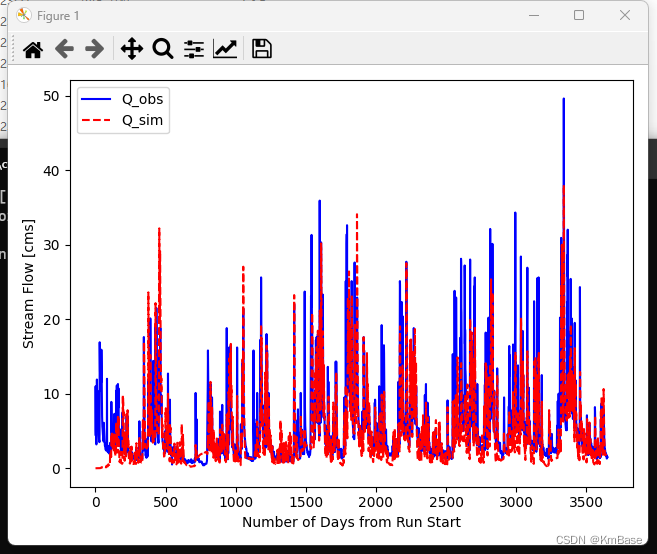
plt.plot(q_obs, label='Q_obs', color='blue')
plt.plot(q_sim, label='Q_sim', color='red', ls='--')
plt.legend(fontsize=10)
plt.ylabel('Stream Flow [cms]', fontsize=10)
plt.xlabel('Number of Days from Run Start', fontsize=10)
plt.tight_layout()
plt.show()
model_error = nse_cost(para_init)
f_out = open('model_err.dat', 'w+')
f_out.write(str(model_error) + '\n')
f_out.close()
if __name__ == '__main__':
# Read Input (Air Temp.,PET, Precip.)
month, temp, precip = np.genfromtxt('inputPrecipTemp.txt', usecols=[1, 2, 3], unpack=True)
monthly, tpem, dpem = np.genfromtxt('inputMonthlyTempEvap.txt', unpack=True)
month = month.astype(int)
# Read Q observed
q_obs = np.genfromtxt('Qobs.txt')
main()
以上代码,运行结果