import numpy as np
from sklearn.linear_model import LogisticRegression
import matplotlib.pyplot as plt
import matplotlib as mpl
from sklearn import preprocessing
import pandas as pd
from sklearn.preprocessing import StandardScaler
from sklearn.pipeline import Pipeline
if __name__ == '__main__':
path = 'iris.data'
data = pd.read_csv('iris.data', header=None)
iris_types = data[4].unique()
for i, type in enumerate(iris_types):
data.set_value(data[4] == type, 4, i)
x, y = np.split(data.values, (4,), axis=1)
x = x.astype(np.float)
y = y.astype(np.int)
print('x = \n', x)
print('y = \n', y)
# 仅使用前两列特征
x = x[:, :2]
lr = Pipeline([('sc', StandardScaler()), ('clf', LogisticRegression())])
lr.fit(x, y.ravel())
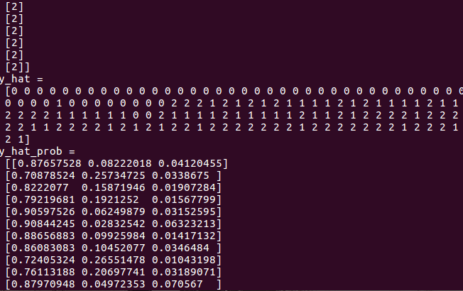
y_hat = lr.predict(x)
y_hat_prob = lr.predict_proba(x)
np.set_printoptions(suppress=True)
print('y_hat = \n', y_hat)
print('y_hat_prob = \n', y_hat_prob)
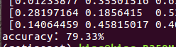
print('accuracy:%.2f%%' % (100*np.mean(y_hat == y.ravel())))
# 画图
# 横纵各采样多少个值
N, M = 1000, 1000
# 第0列的范围
x1_min, x1_max = x[:, 0].min(), x[:, 0].max()
# 第1列的范围
x2_min, x2_max = x[:, 1].min(), x[:, 1].max()
t1 = np.linspace(x1_min, x1_max, N)
t2 = np.linspace(x2_min, x2_max, M)
# 生成网格采样点
x1, x2 = np.meshgrid(t1, t2)
# 测试点
x_test = np.stack((x1.flat, x2.flat), axis=1)
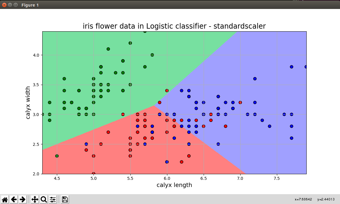
cm_light = mpl.colors.ListedColormap(['#77E0A0', '#FF8080', '#A0A0FF'])
cm_dark = mpl.colors.ListedColormap(['g', 'r', 'b'])
# 预测值
y_hat = lr.predict(x_test)
# 使之与输入的形状相同
y_hat = y_hat.reshape(x1.shape)
plt.figure(facecolor='w')
# 预测值的显示
plt.pcolormesh(x1, x2, y_hat, cmap=cm_light)
# 样本的显示
plt.scatter(x[:, 0], x[:, 1], c=np.squeeze(y), edgecolors='k', s=50, cmap=cm_dark)
plt.xlabel('calyx length', fontsize=14)
plt.ylabel('calyx width', fontsize=14)
plt.xlim(x1_min, x1_max)
plt.ylim(x2_min, x2_max)
plt.grid()
plt.title('iris flower data in Logistic classifier - standardscaler', fontsize=17)
plt.show()