分布式估计器
定义系统参数
参考文献:https://ieeexplore.ieee.org/document/9750909
import numpy as np

# 状态个数
n = 4
# 传感器个数
N = 7
# 每个传感器的信息
ri = 1
# 状态矩阵,n*n
A = np.array([[0.1,     0,      -0.1,   0],
              [-0.2,    -0.1,   0,      0],
              [0,       0,      0.2,    0.2],
              [-0.1,    0,      0,      -0.3]
              ])
# 输出矩阵,N*n
C = np.array([[0,   2.0,  0,    0],
              [0,   0,    1.5,  0],
              [1.0, 0,    0,    0],
              [0,   0,    2.0,  0],
              [1.0, 0,    0,    0],
              [0,   0,    0,    2.0],
              [1.0, 0,    0,    0],
              ])
# 噪声转移矩阵,ri*ri
Phi=[]
for i in range(N):
    Phi.append(np.array([-0.20 + 0.010 * (i+1)]))
Phi = np.concatenate(Phi)
# 噪声协方差
Q=np.eye(n)
R=0.1*np.ones([N,ri])
# 初值
x_0=2*np.ones([n,ri])
P_0=np.eye(n)
z_0=0.5 #*np.ones([N,ri])
# 领接矩阵
Adj=np.array([[1,   1,   0,   0,   0,   0,   1],
              [1,   1,   1,   0,   0,   0,   0],
              [0,   1,   1,   1,   0,   0,   0],
              [0,   0,   1,   1,   1,   0,   0],
              [0,   0,   0,   1,   1,   1,   0],
              [0,   0,   0,   0,   1,   1,   1],
              [1,   0,   0,   0,   0,   1,   1],
              ])
# 打印结果
print("Phi:\n", Phi)
print("Q:\n", Q)
print("R:\n", R)
print("z_0:\n", z_0)
print("x_0:\n", x_0)
print("Adj:\n", Adj)
B=np.dot(-C.T,np.dot(np.linalg.inv(np.diag([item for sublist in R for item in sublist])), C))
B
根据公式(5)~(8)
首先求解方程 A P + P A T + P B P = − Q AP + PA^T+PBP=-Q AP+PAT+PBP=−Q
其中, B = − C T R z − 1 C B=-C^TR_z^{-1}C B=−CTRz−1C
参考https://zhuanlan.zhihu.com/p/24893371
得到两种解
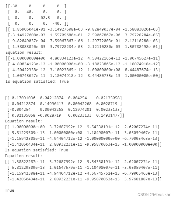
选择第一种解,因为第二种值太大了
from scipy.optimize import fsolve
B=np.dot(-C.T,np.dot(np.linalg.inv(np.diag([item for sublist in R for item in sublist])), C))
print(B)

# 方程AP + PA^T+PBP=-Q
def func(P):
    P = P.reshape(n, n)
    matrix = np.dot(A, P) + np.dot(P, A.T) + np.dot(P, np.dot(B, P)) + Q
    # 将[[1] [2] [3] [4]],转成[1,2,3,4]
    flat_list = [item for sublist in matrix for item in sublist]
    return flat_list

P = fsolve(func,[1, 0, 0, 0,
                 0, 0, 0, 0,
                 0, 0, 1, 0,
                 0, 0, 0, 1])

P = P.reshape(n, n)
print(P)

# 验证结果
eqn_result = np.dot(A, P) + np.dot(P, A.T) + np.dot(P, np.dot(B, P))
print("Equation result:")
print(eqn_result)
print("Is equation satisfied:", np.allclose(eqn_result, -Q))
residual = np.dot(A, P) + np.dot(P, A.T) + np.dot(P, np.dot(B, P)) + Q
is_correct = np.allclose(residual, np.zeros_like(residual))
print("Equation result:")
print(residual)
is_correct
ξ i j \xi_{ij} ξij是传感器j对于传感器i的测量估计
![[外链图片转存失败,源站可能有防盗链机制,建议将图片保存下来直接上传(img-JkYDUyrm-1689236960924)(attachment:image.png)]](https://img-blog.csdnimg.cn/743eda4e8dc54c00a022d6444a8e7e39.png)
ξij(0) = Cj x0
Cj是C矩阵的第j行
#  the estimator gain 矩阵 n * N
K = - np.dot(P, np.dot(C.T, np.linalg.inv(np.diag([item for sublist in R for item in sublist])) ))
print("K:\n", K)
mu = 8  #2 * (1 - np.cos(np.pi / N))    # 可修改
# 初值
#
y0=[]
for i in range(N):
    y0.append(np.dot(C[i], x_0))
print([item for sublist in y0 for item in sublist])
xi_0 = np.zeros_like(Adj)
for i in range(N):
    for j in range(N):
        if Adj[i][j]==1:
            xi_0[j][i]=np.dot(C[j],x_0)
        else:
            xi_0[j][i]=0
# xi_0=Adj
print(xi_0)
print(xi_0[:,0])
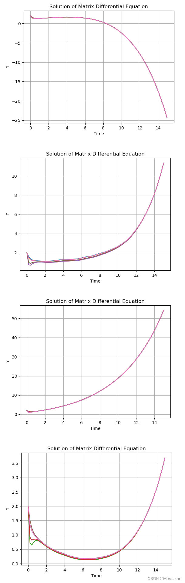
求解微分方程
# 求解微分方程
import numpy as np
from scipy.integrate import solve_ivp
import matplotlib.pyplot as plt

mu = 10 #2 * (1 - np.cos(np.pi / N))    # 可修改


t_sum=15 # 秒
t_span = (0, t_sum)  # 时间范围
t = np.linspace(0, t_sum, 77)  # 用于绘制的时间点
# 设置随机种子,以便结果可复现
np.random.seed(0)
# 生成白噪声
white_noise = np.random.normal(0, 0.005, size=len(t))
# 生成维纳过程
wiener_process = np.cumsum(white_noise)

def white_noise_fun(target):
    closest_index = min(range(len(t)), key=lambda i: abs(t[i] - target))
    res= white_noise[closest_index]
    return res

def wiener_process_fun(target):
    closest_index = min(range(len(t)), key=lambda i: abs(t[i] - target))
    res= wiener_process[closest_index]
    return res

def matrix_differential_equation(tt, X):
    x_hat = X[:n*N]
    xi = X[n*N:]
    x_hat = x_hat.reshape([N,n])# 都横着吧
    xi = xi.reshape([N,N])
    y = np.array([])
    for i in range(N):
        # y = np.append(y, np.dot(C[i], x_hat[i])) # + z_0   # 之后再加噪声
        # y = np.append(y, np.dot(C[i], x_hat[i])) + white_noise_fun(tt);   # + z_0
        y = np.append(y, np.dot(C[i], x_hat[i])) + wiener_process_fun(tt)    # + z_0
    dot_x_hat = np.array([])
    dot_xi = np.array([])
    for i in range(N):
        temp = np.dot(A + np.dot(K, C) , x_hat[i]) - np.dot(K, xi[i])
        dot_x_hat = np.append(dot_x_hat, temp)
        sum_N = np.zeros([1,N])
        for k in range(N):
            sum_N = sum_N + Adj[i][k] * (xi[i]-xi[k])
        dd=-mu *(sum_N + np.dot(np.diag(Adj[:,i]) , (xi[i] - y))) + np.dot(np.dot(C, A) , x_hat[i])
        dot_xi =np.append(dot_xi, dd)
    dX_dt=np.array([])
    dX_dt=np.append(dX_dt,dot_x_hat)
    dX_dt=np.append(dX_dt,dot_xi)
    return dX_dt

# 微分方程的初值

X = np.array([])
for i in range(N):
    X=np.append(X,x_0.reshape(n))
X=np.append(X,xi_0.reshape(N*N))
print(X)
initial_condition = X  # 初始条件

solution = solve_ivp(matrix_differential_equation, t_span, initial_condition, dense_output=True)

Y = solution.sol(t)
print(len(t))

for k in range(n):
    for i in range(N):
        plt.plot(t, Y[i*n+k,:])
    plt.xlabel('Time')
    plt.ylabel('Y')
    plt.title('Solution of Matrix Differential Equation')
    # plt.legend()
    plt.grid(True)
    plt.show()
得到的结果图如下:
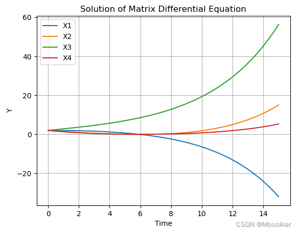
和真实的状态相比较
# 初值

t_sum=15 # 秒
t_span = (0, t_sum)  # 时间范围
t = np.linspace(0, t_sum, 77)  # 用于绘制的时间点

def origin(tt, X):
    dX_dt = np.dot(A, X)#+ wiener_process_fun(tt)  # 计算微分方程的导数
    return dX_dt

initial_condition = np.array([2, 2, 2, 2])  # 初始条件

solution = solve_ivp(origin, t_span, initial_condition, dense_output=True)

X = solution.sol(t)

plt.plot(t, X[0], label='X1')
plt.plot(t, X[1], label='X2')
plt.plot(t, X[2], label='X3')
plt.plot(t, X[3], label='X4')
plt.xlabel('Time')
plt.ylabel('Y')
plt.title('Solution of Matrix Differential Equation')
plt.legend()
plt.grid(True)
plt.show()
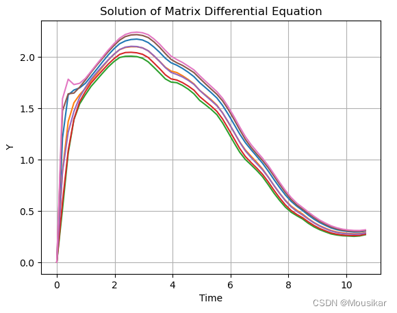
求解均方差
M S E i ( t ) = ∣ ∣ x ( t ) − x ^ i ( t ) ∣ ∣ 2 2 MSE_i(t)=||x(t)-\hat x_i (t)||_2^2 MSEi(t)=∣∣x(t)−x^i(t)∣∣22
MSE=[]
len(Y[i*n+2,:])
len(X[2])
np.mean((Y[i*n+2,:] - X[2]) ** 2)
for j in range(len(X[2])):
    temp=[]
    for i in range(N):
        aaa=np.mean(( X[2,j] - Y[i*n+2,j]) ** 2)
        temp.append(aaa)
    MSE.append(temp)
len(MSE)
MSE = np.array(MSE)
for i in range(N):
    plt.plot(t[:55], MSE[:55,i])
plt.xlabel('Time')
plt.ylabel('Y')
plt.title('Solution of Matrix Differential Equation')
# plt.legend()
plt.grid(True)
plt.show()
源文件可以在这里找到:https://download.csdn.net/download/weixin_45226065/88046590