数据和相关性计算
数据是内置的,为phylsoeq对象,大家自己导入如果不会操作,可以在网上直接搜索:
rm(list=ls())
library(ggClusterNet)
library(tidyverse)
library(phyloseq)
#----------计算相关#----
result = cor_Big_micro(ps = ps,
                       N = 2000,
                       # method.scale = "TMM",
                       r.threshold=0.5,
                       p.threshold=0.05,
                       method = "spearman"
)

#--提取相关矩阵
cor = result[[1]]
model_Gephi.3算法
#--使用model Gephi3算法展示网络#------
tab = model_Gephi.3(
  cor = cor,
  t0 = 0.98, # 取值范围为0到1,表示位于两个已知点之间的中间位置
  t2 = 1.2, # 每个聚类中心的缩放
  t3 = 8) # 聚类取哪个点,数值越大,取点越靠近00点

tem3 = tab[[1]]
node.p = tab[[2]]
head(tem3)
aa = node.p$group %>% table() %>% as.data.frame() %>%
  rename(  "group" = ".")

tid = aa$group[aa$Freq < 60] %>% as.character()
tem3$group = as.character(tem3$group)
tem3$group[(tem3$group) %in% tid] = "miniModule"
test_color5 <- RColorBrewer::brewer.pal(n = 12,name = "Set3")
head(tem3)
tem3$ID = NULL
colnames(tem3)[5] = "Group"
head(node.p)

nodef = node.p %>% left_join(tem3,by = c("ID" = "OTU"))
head(nodef)
邓老师GCB文章结果网络布局算法复现
#-邓老师GCB文章结果复现#-----

p2 <- ggplot() +
  # geom_segment(aes(x = X1, y = Y1, xend = X2, yend = Y2,color = as.factor(cor)),
  #                               data = edge, size = 0.5,alpha = 0.01) +
  geom_point(aes(X1, X2,fill = Group),pch = 21, data = nodef,
             color= "white",size = 6
  ) +
  scale_colour_brewer(palette = "Set1") +
  scale_fill_hue() +
  scale_fill_manual(values  =
                      c(
                        "#4DAF4A","#A65628","#FDAE61" ,"#FEE08B","#3288BD","grey80","grey90")
  )+
  scale_x_continuous(breaks = NULL) +
  scale_y_continuous(breaks = NULL) +
  scale_size(range = c(3, 20)) +
  # labs( title = paste(layout,"network",sep = "_"))+
  # geom_text_repel(aes(X1, X2,label=Phylum),size=4, data = plotcord)+
  # discard default grid + titles in ggplot2
  theme(panel.background = element_blank()) +
  # theme(legend.position = "none") +
  theme(axis.title.x = element_blank(), axis.title.y = element_blank()) +
  theme(legend.background = element_rect(colour = NA)) +
  theme(panel.background = element_rect(fill = "white",  colour = NA)) +
  theme(panel.grid.minor = element_blank(), panel.grid.major = element_blank())
p2

ggsave("cs0.pdf",p2,width = 15,height = 14)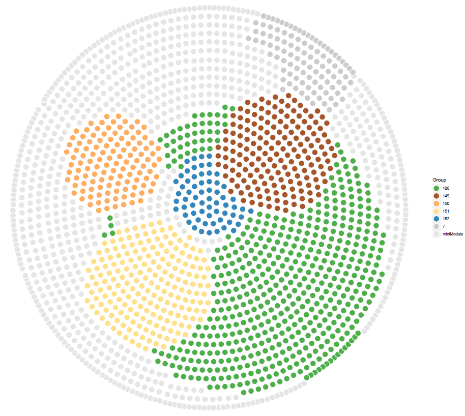
使用模块度进行填充
#--使用大小填充#-----

p2 <- ggplot() +
  # geom_segment(aes(x = X1, y = Y1, xend = X2, yend = Y2,color = as.factor(cor)),
  #                               data = edge, size = 0.5,alpha = 0.01) +
  geom_point(aes(X1, X2,fill = Group,
                 size = igraph.degree),pch = 21, data = nodef,color= "grey80"
  ) +
  scale_colour_brewer(palette = "Set1") +
  scale_fill_hue() +
  scale_fill_manual(values  =
                      c(
                        "#4DAF4A","#A65628","#FDAE61" ,"#FEE08B","#3288BD","grey80","grey90")
  )+
  scale_x_continuous(breaks = NULL) +
  scale_y_continuous(breaks = NULL) +
  scale_size(range = c(3, 20)) +
  # labs( title = paste(layout,"network",sep = "_"))+
  # geom_text_repel(aes(X1, X2,label=Phylum),size=4, data = plotcord)+
  # discard default grid + titles in ggplot2
  theme(panel.background = element_blank()) +
  # theme(legend.position = "none") +
  theme(axis.title.x = element_blank(), axis.title.y = element_blank()) +
  theme(legend.background = element_rect(colour = NA)) +
  theme(panel.background = element_rect(fill = "white",  colour = NA)) +
  theme(panel.grid.minor = element_blank(), panel.grid.major = element_blank())
p2

ggsave("cs1.pdf",p2,width = 20,height = 19)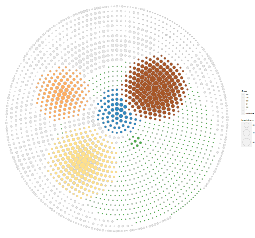
展示节点扰动对布局样式的影响
library(igraph)

#--展示扰动点对聚类布局的影响#----------
plots = list()
id = c(0,0.2,0.4,0.6,0.8,1)
for (j in 1:length(id)) {
  i = id[j]
  tab = model_Gephi.3(
    cor = cor,
    t0 = 0.98, # 取值范围为0到1,表示位于两个已知点之间的中间位置
    t2 = 1.2, # 每个聚类中心的缩放
    t3 = 8) # 聚类取哪个点,数值越大,取点越靠近00点

  tem3 = tab[[1]]
  node.p = tab[[2]]
  head(tem3)

  aa = node.p$group %>% table() %>% as.data.frame() %>%
    rename(  "group" = ".")

  tid = aa$group[aa$Freq < 60] %>% as.character()
  tem3$group = as.character(tem3$group)
  tem3$group[(tem3$group) %in% tid] = "miniModule"
  test_color5 <- RColorBrewer::brewer.pal(n = 12,name = "Set3")
  head(tem3)
  tem3$ID = NULL
  colnames(tem3)[5] = "Group"
  head(node.p)

  nodef = node.p %>% left_join(tem3,by = c("ID" = "OTU"))
  head(nodef)

  p2 <- ggplot() +
    # geom_segment(aes(x = X1, y = Y1, xend = X2, yend = Y2,color = as.factor(cor)),
    #                               data = edge, size = 0.5,alpha = 0.01) +
    geom_point(aes(X1, X2,fill = Group,size = igraph.degree),pch = 21, data = nodef,color= "grey80",
               position=position_jitter(width=i,height=i)
    ) +
    scale_colour_brewer(palette = "Set1") +
    scale_fill_hue() +
    scale_fill_manual(values  =
                        c(
                          "#4DAF4A","#A65628","#FDAE61" ,"#FEE08B" ,"#3288BD","grey80","grey90")
    )+
    scale_x_continuous(breaks = NULL) +
    scale_y_continuous(breaks = NULL) +
    scale_size(range = c(3, 20)) +
    # labs( title = paste(layout,"network",sep = "_"))+
    # geom_text_repel(aes(X1, X2,label=Phylum),size=4, data = plotcord)+
    # discard default grid + titles in ggplot2
    theme(panel.background = element_blank()) +
    # theme(legend.position = "none") +
    theme(axis.title.x = element_blank(), axis.title.y = element_blank()) +
    theme(legend.background = element_rect(colour = NA)) +
    theme(panel.background = element_rect(fill = "white",  colour = NA)) +
    theme(panel.grid.minor = element_blank(), panel.grid.major = element_blank())
  p2
  plots[[j]] = p2
}

p1  = ggpubr::ggarrange(plotlist = plots,
                        common.legend = FALSE, legend="right",ncol = 3,nrow = 2)
p1
ggsave("cs2.pdf",p1,width = 20*3,height = 19*2,limitsize = FALSE)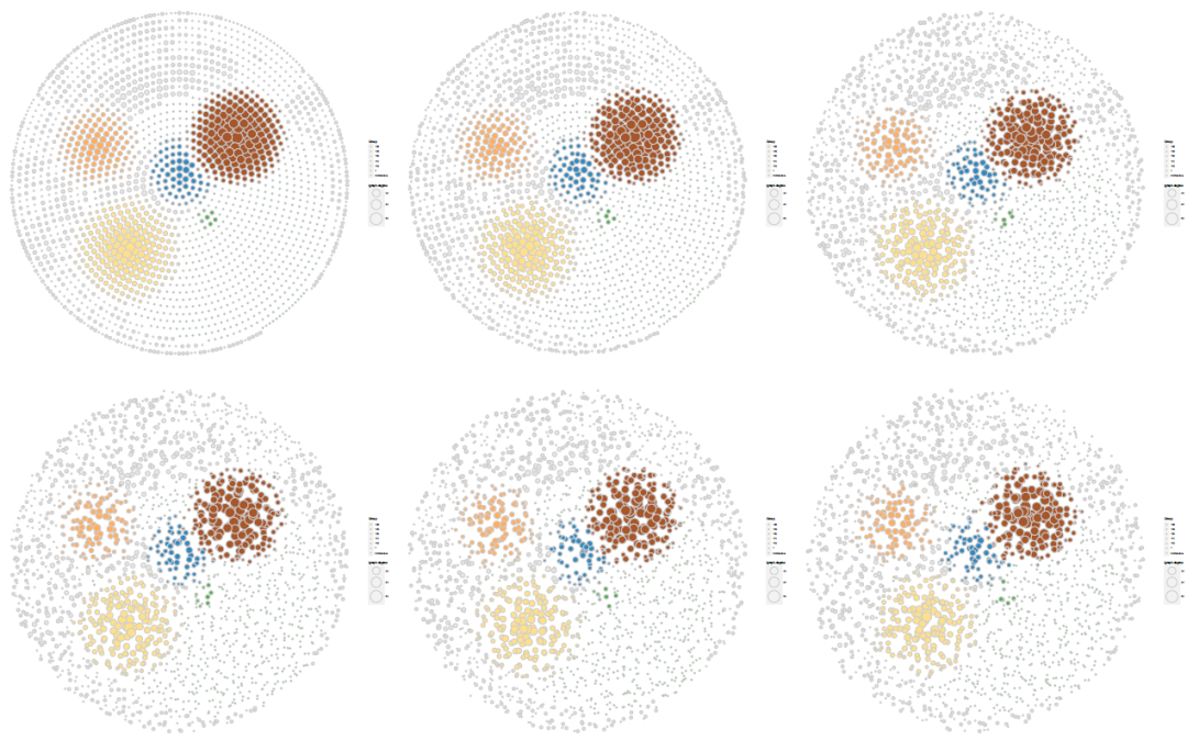
展示模块游动对网络布局的影响
#--展示游动模块#-----
plots = list()

id = c(1,1.5,2,2.5,3.0,3.5,4)

for (j in 1:length(id)) {

  i = 0.2
  tab = model_Gephi.3(
    cor = cor,
    t0 = 0.98, # 取值范围为0到1,表示位于两个已知点之间的中间位置
    t2 = id[j], # 每个聚类中心的缩放
    t3 = 8) # 聚类取哪个点,数值越大,取点越靠近00点


  tem3 = tab[[1]]
  node.p = tab[[2]]
  head(tem3)


  aa = node.p$group %>% table() %>% as.data.frame() %>%
    rename(  "group" = ".")

  tid = aa$group[aa$Freq < 60] %>% as.character()
  tem3$group = as.character(tem3$group)
  tem3$group[(tem3$group) %in% tid] = "miniModule"
  test_color5 <- RColorBrewer::brewer.pal(n = 12,name = "Set3")
  head(tem3)
  tem3$ID = NULL
  colnames(tem3)[5] = "Group"
  head(node.p)

  nodef = node.p %>% left_join(tem3,by = c("ID" = "OTU"))
  head(nodef)

  # p1 <- ggplot() +
  #   # geom_segment(aes(x = X1, y = Y1, xend = X2, yend = Y2),
  #   #                             data = edge, size = 1) +
  #   geom_point(aes(X1, X2,fill = group), data = tem3,pch = 21,
  #              position=position_jitter(width=0.15,height=0.15)
  #
  #              ) +
  #   theme_void()
  # p1

  # "#E41A1C" "#377EB8" "#4DAF4A" "#984EA3" "#FF7F00" "#FFFF33" "#A65628" "#F781BF" "#999999"
  p2 <- ggplot() +
    # geom_segment(aes(x = X1, y = Y1, xend = X2, yend = Y2,color = as.factor(cor)),
    #                               data = edge, size = 0.5,alpha = 0.01) +
    geom_point(aes(X1, X2,fill = Group,size = igraph.degree),pch = 21, data = nodef,color= "grey80",
               position=position_jitter(width=i,height=i)
    ) +
    scale_colour_brewer(palette = "Set1") +
    scale_fill_hue() +
    scale_fill_manual(values  =
                        c(
                          "#4DAF4A","#A65628","#FDAE61" ,"#FEE08B" ,"#3288BD","grey80","grey90")
    )+
    scale_x_continuous(breaks = NULL) +
    scale_y_continuous(breaks = NULL) +
    scale_size(range = c(3, 20)) +
    # labs( title = paste(layout,"network",sep = "_"))+
    # geom_text_repel(aes(X1, X2,label=Phylum),size=4, data = plotcord)+
    # discard default grid + titles in ggplot2
    theme(panel.background = element_blank()) +
    # theme(legend.position = "none") +
    theme(axis.title.x = element_blank(), axis.title.y = element_blank()) +
    theme(legend.background = element_rect(colour = NA)) +
    theme(panel.background = element_rect(fill = "white",  colour = NA)) +
    theme(panel.grid.minor = element_blank(), panel.grid.major = element_blank())
  p2
  plots[[j]] = p2
}

p1  = ggpubr::ggarrange(plotlist = plots,
                        common.legend = FALSE, legend="right",ncol = 4,nrow = 2)
p1
ggsave("cs3.pdf",p1,width = 20*4,height = 19*2,limitsize = FALSE)根际互作生物学研究室 简介根际互作生物学研究室是沈其荣院士土壤微生物与有机肥团队下的一个关注于根际互作的研究小组。本小组由袁军副教授带领,主要关注:1.植物和微生物互作在抗病过程中的作用;2 环境微生物大数据整合研究;3 环境代谢组及其与微生物过程研究体系开发和应用。团队在过去三年中在 Nature Communication,ISME J,Microbiome,SCLS,New Phytologist,iMeta,Fundamental Research, PCE,SBB,JAFC(封面),Horticulture Research,SEL(封面),BMC plant biology等期刊上发表了多篇文章。欢迎关注 微生信生物 公众号对本研究小组进行了解。
撰写:文涛
修改:文涛
审核:袁军
团队工作及其成果 (点击查看)了解 交流 合作-
团队成员邮箱 袁军:[email protected];文涛:[email protected]
团队公众号:微生信生物 添加主编微信,或者后台留言。
点击查看团队github主页
点击查看南京农业大学资源于环境科学学院主页
加主编微信 加入群聊
目前营销人员过多,为了维护微生信生物3年来维护的超5000人群聊,目前更新进群要求:
1.仅限相关专业或研究方向人员添加,必须实名,不实名则默认忽略。
2.非相关专业的其他人员及推广宣传人员禁止添加。
3.添加主编微信需和简单聊一聊专业相关问题,等待主编判断后,可拉群。
4 微生信生物VIP微信群不受限制,费用为60一位,红包发主编即可(群里发送推文代码+高效协助解决推文运行等问题+日常问题咨询回复)。