UNet算法原理解读及paddle实现
U-Net网络是一个非常经典的图像分割网络,起源于医疗图像分割,具有参数少、计算快、应用性强的特点,对于一般场景适应度很高。U-Net最早于2015年提出,并在ISBI 2015 Cell Tracking Challenge取得了第一。
U-Net的结构是标准的编码器-解码器结构,如 图1 所示。左侧可视为一个编码器,右侧可视为一个解码器。图像先经过编码器进行下采样得到高级语义特征图,再经过解码器上采样将特征图恢复到原图片的分辨率。网络中还使用了跳跃连接,即解码器每上采样一次,就以拼接的方式将解码器和编码器中对应相同分辨率的特征图进行特征融合,帮助解码器更好地恢复目标的细节。
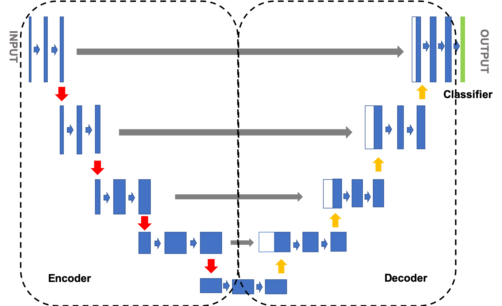
1)Encoder:编码器整体呈现逐渐缩小的结构,不断缩小特征图的分辨率,以捕获上下文信息。编码器共分为4个阶段,在每个阶段中,使用最大池化层进行下采样,然后使用两个卷积层提取特征,最终的特征图缩小了16倍;
2)Decoder:解码器呈现与编码器对称的扩张结构,逐步修复分割对象的细节和空间维度,实现精准的定位。解码器共分为4个阶段,在每个阶段中,将输入的特征图进行上采样后,与编码器中对应尺度的特征图进行拼接运算,然后使用两个卷积层提取特征,最终的特征图放大了16倍;
3)分类模块:使用大小为3×3的卷积,对像素点进行分类;
说明:
延伸阅读:U-Net: Convolutional Networks for Biomedical Image Segmentation
UNet的实现方案如 图2 所示,对于一幅宠物图像,首先使用卷积神经网络UNet网络中的编码器提取特征(包含4个下采样阶段),获取高级语义特征图;然后使用解码器(包含4个上采样阶段)将特征图恢复到原始尺寸。在训练阶段,通过模型输出的预测图与样本的真实标签图构建损失函数,从而进行模型训练;在推理阶段,使用模型的预测图作为最终的输出。
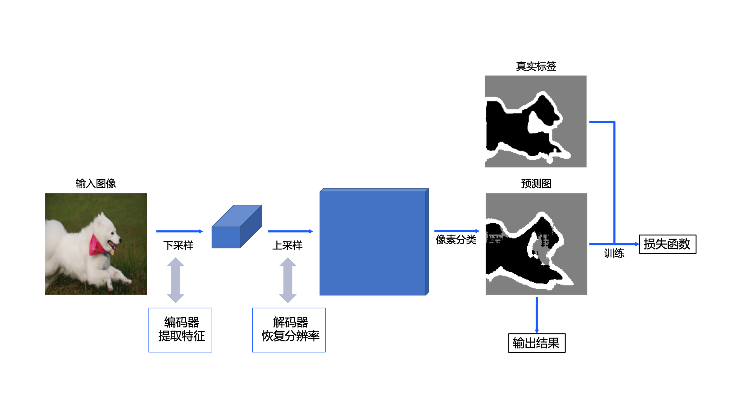
图2 宠物图像分割设计方案
整体的U-Net网络框架代码实现如下所示:
# coding=utf-8
# 导入环境
import os
import random
import cv2
import numpy as np
from PIL import Image
from paddle.io import Dataset
import matplotlib.pyplot as plt
# 在notebook中使用matplotlib.pyplot绘图时,需要添加该命令进行显示
%matplotlib inline
import paddle
import paddle.nn.functional as F
import paddle.nn as nn

class UNet(nn.Layer):
    # 继承paddle.nn.Layer定义网络结构
    def __init__(self, num_classes=3):
        # 初始化函数
        super().__init__()
        # 定义编码器
        self.encode = Encoder()
        # 定义解码器
        self.decode = Decoder()
        # 分类模块
        self.cls = nn.Conv2D(in_channels=64, out_channels=num_classes, kernel_size=3, stride=1, padding=1)

    def forward(self, x):
        # 前向计算
        logit_list = []
        # 编码运算
        x, short_cuts = self.encode(x)
        # 解码运算
        x = self.decode(x, short_cuts)
        # 分类运算
        logit = self.cls(x)
        logit_list.append(logit)
        return logit_list
定义编码器
上边我们将模型分为了编码器、解码器和分类模块三个部分。其中,分类模块已经被实现,接下来分别定义编码器和解码器部分:
首先是编码器部分。这里的编码器通过不断地重复一个单元结构来增加通道数,减小图片尺寸,得到高级语义特征图。
代码实现如下所示:
class ConvBNReLU(nn.Layer):
    def __init__(self, in_channels, out_channels, kernel_size, padding='same'):
        # 初始化函数
        super().__init__()
        # 定义卷积层
        self._conv = nn.Conv2D(in_channels, out_channels, kernel_size, padding=padding)
        # 定义批归一化层
        self._batch_norm = nn.SyncBatchNorm(out_channels)

    def forward(self, x):
        # 前向计算
        x = self._conv(x)
        x = self._batch_norm(x)
        x = F.relu(x)
        return x
class Encoder(nn.Layer):
    def __init__(self):
        # 初始化函数
        super().__init__()
        # # 封装两个ConvBNReLU模块
        self.double_conv = nn.Sequential(ConvBNReLU(3, 64, 3), ConvBNReLU(64, 64, 3))
        # 定义下采样通道数
        down_channels = [[64, 128], [128, 256], [256, 512], [512, 512]]
        # 封装下采样模块
        self.down_sample_list = nn.LayerList([self.down_sampling(channel[0], channel[1]) for channel in down_channels])

    # 定义下采样模块
    def down_sampling(self, in_channels, out_channels):
        modules = []
        # 添加最大池化层
        modules.append(nn.MaxPool2D(kernel_size=2, stride=2))
        # 添加两个ConvBNReLU模块
        modules.append(ConvBNReLU(in_channels, out_channels, 3))
        modules.append(ConvBNReLU(out_channels, out_channels, 3))
        return nn.Sequential(*modules)

    def forward(self, x):
        # 前向计算
        short_cuts = []
        # 卷积运算
        x = self.double_conv(x)
        # 下采样运算
        for down_sample in self.down_sample_list:
            short_cuts.append(x)
            x = down_sample(x)
        return x, short_cuts
定义解码器
在通道数达到最大,得到高级语义特征图后,网络结构会开始进行解码操作。这里的解码也就是进行上采样,减小通道数的同时逐步增加对应图片尺寸,直至恢复到原图像大小。本实验中,使用双线性插值方法实现图片的上采样。
具体代码如下所示:
# 定义上采样模块
class UpSampling(nn.Layer):
    def __init__(self, in_channels, out_channels):
        # 初始化函数
        super().__init__()
        in_channels *= 2
        # 封装两个ConvBNReLU模块
        self.double_conv = nn.Sequential(ConvBNReLU(in_channels, out_channels, 3), ConvBNReLU(out_channels, out_channels, 3))

    def forward(self, x, short_cut):
        # 前向计算
        # 定义双线性插值模块
        x = F.interpolate(x, paddle.shape(short_cut)[2:], mode='bilinear')
        # 特征图拼接
        x = paddle.concat([x, short_cut], axis=1)
        # 卷积计算
        x = self.double_conv(x)
        return x
# 定义解码器
class Decoder(nn.Layer):
    def __init__(self):
        # 初始化函数
        super().__init__()
        # 定义上采样通道数
        up_channels = [[512, 256], [256, 128], [128, 64], [64, 64]]
        # 封装上采样模块
        self.up_sample_list = nn.LayerList([UpSampling(channel[0], channel[1]) for channel in up_channels])

    def forward(self, x, short_cuts):
        # 前向计算
        for i in range(len(short_cuts)):
            # 上采样计算
            x = self.up_sample_list[i](x, short_cuts[-(i + 1)])
        return x