线性回归的基本要素:
模型(学习模型参数 权重weight,偏差bias)
训练数据
损失函数(需要对比模型的输出和真实值之间的误差。损失函数可以衡量输出结果对比真实数据的好坏。)
优化算法(需要算法来通盘考虑模型本身和损失函数,对参数进行搜索,从而逐渐最小化损失。最常见的神经网络优化使用梯度下降法作为优化算法。简单地说,轻微地改动参数,观察训练集的损失将如何移动。然后将参数向减小损失的方向调整。)
线性回归的表示方法:
神经网络图
输⼊分别为 x1 和 x2,因此输⼊层的输⼊个数为 2。输⼊个数也叫特征数或特征向量维度。由于⽹络的输出为 o,输出层的输出个数为 1。图 中神经⽹络的输出 o 作为线性回归的输出,即 yˆ = o。由于输⼊层并不涉及计算,神经⽹络的层数为 1。所以,线性回归是⼀个单层神经⽹络。输出层中负责计算 o 的单元⼜叫神经元。在线性回归中,o 的计算依赖于 x1 和 x2。也就是说,输出层中的神经元和输⼊层中各个输⼊完全连接。因此,这⾥的输出层⼜叫全连接层或稠密层(fully-connectedlayer 或 dense layer)。

扫描二维码关注公众号,回复:
1644558 查看本文章

矢量计算表达式
#在深度学习中要尽可能使用矢量计算,以提升计算效率
from mxnet import nd
from time import time


a=nd.ones(shape=1000)
b=nd.ones(shape=1000)

#mxnet中测试时间方法
start = time()
c = nd.zeros(shape=1000)
for i in range(1000):
    c[i]=a[i]+b[i]
t1=time()-start

print(t1)

start = time()
d=a+b
t2=time()-start
print(t2)
线性回归:
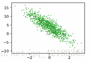
features[:,0]代表第一列,features[:,1]代表第二列
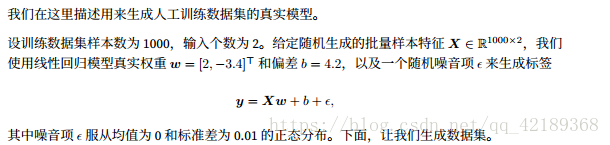
from matplotlib import pyplot as plt
from mxnet import autograd,nd
import random

#使用人工训练数据训练模型
num_inputs=2
num_examples=1000
true_w=[2,-3.4]
true_b=4.2

features=nd.random.normal(scale=1,shape=(num_examples,num_inputs))
labels=true_w[0]*features[:,0]+true_w[1]*features[:,1]+true_b
labels+=nd.random.normal(scale=0.01,shape=labels.shape)

#显示训练数据
features[0],labels[0]


%config InlineBackend.figure_format='retina'

plt.rcParams['figure.figsize']=(3.5,2.5)
plt.scatter(features[:, 1].asnumpy(),labels.asnumpy(),1)
plt.show()
indices:产生一个随机索引值
yield:每次读取一个数值
#读取数据
#训练模型时,需要遍历数据不断读取小批量数据样本。
batch_size = 10
def data_iter(batch_size, num_examples, features, labels):
indices = list(range(num_examples))
random.shuffle(indices)
for i in range(0, num_examples, batch_size):
j = nd.array(indices[i: min(i + batch_size, num_examples)])
yield features.take(j), labels.take(j)
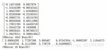
for X, y in data_iter(batch_size, num_examples, features, labels):
print(X, y)
break
#初始化模型参数
w = nd.random.normal(scale=0.01, shape=(num_inputs, 1))
b = nd.zeros(shape=(1,))
params = [w, b]
for param in params:
    param.attach_grad()
#定义模型
def linreg(X, w, b):
    return nd.dot(X, w) + b

#定义损失函数
def squared_loss(y_hat, y):
    return (y_hat - y.reshape(y_hat.shape)) ** 2 / 2

#定义优化算法
def sgd(params, lr, batch_size):
    for param in params:
        param[:] = param - lr * param.grad / batch_size

#训练模型
lr = 0.03
num_epochs = 3
net = linreg
loss = squared_loss

for epoch in range(1, num_epochs + 1):
    for X, y in data_iter(batch_size, num_examples, features, labels):
        with autograd.record():
            l = loss(net(X, w, b), y)
        l.backward()
        sgd([w, b], lr, batch_size)
    print("epoch %d, loss %f"
          % (epoch, loss(net(features, w, b), labels).mean().asnumpy()))

参考:
1.https://github.com/mli/gluon-tutorials-zh