题目链接:点击打开链接
这篇博客只是实现了单变量线性回归,多变量的内容在下一篇博客中展现。
首先表述下文符号的含义
m = 训练样本的数量
x = 输入变量/特征
y = 输出变量/目标变量
(x,y) = 训练样本
= 第i个样本
首先展示几个学到的公式:
1.假设函数
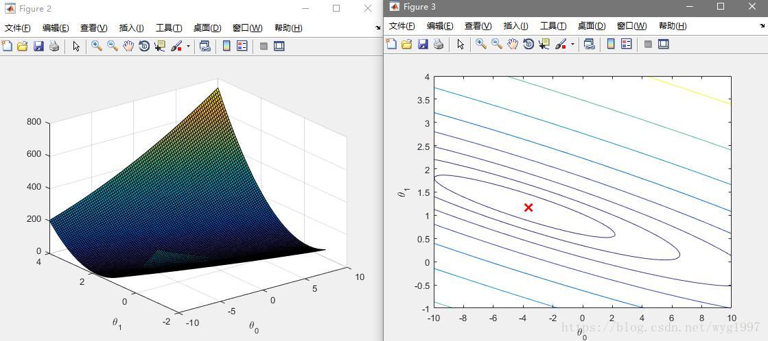
2.代价函数
3.梯度下降法
注意:这里要实现同步更新
然后是代码:
computeCost.m
function J = computeCost(X, y, theta)
%COMPUTECOST Compute cost for linear regression
%   J = COMPUTECOST(X, y, theta) computes the cost of using theta as the
%   parameter for linear regression to fit the data points in X and y

% Initialize some useful values
m = length(y); % number of training examples

% You need to return the following variables correctly
J = 0;

% ====================== YOUR CODE HERE ======================
% Instructions: Compute the cost of a particular choice of theta
%               You should set J to the cost.

%这个方法计算不好
%temp = X * theta;
%temp = temp - y;
%temp = temp.^2;
%J = sum(temp)/2.0/m;

%可以优化成这样
temp = X*theta-y;
J = temp'*temp/2.0/m;

% =========================================================================

end
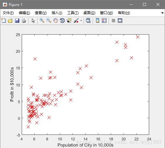
plotData.m
function plotData(x, y)
%PLOTDATA Plots the data points x and y into a new figure
%   PLOTDATA(x,y) plots the data points and gives the figure axes labels of
%   population and profit.

figure; % open a new figure window

% ====================== YOUR CODE HERE ======================
% Instructions: Plot the training data into a figure using the
%               "figure" and "plot" commands. Set the axes labels using
%               the "xlabel" and "ylabel" commands. Assume the
%               population and revenue data have been passed in
%               as the x and y arguments of this function.
%
% Hint: You can use the 'rx' option with plot to have the markers
%       appear as red crosses. Furthermore, you can make the
%       markers larger by using plot(..., 'rx', 'MarkerSize', 10);

plot(x, y, 'rx', 'MarkerSize', 10);  % Plot the data
ylabel('Profit in $10,000s');        % Set the y−axis label
xlabel('Population of City in 10,000s');     % Set the x−axis label

% ============================================================

end
gradientDescent.m
function [theta, J_history] = gradientDescent(X, y, theta, alpha, num_iters)
%GRADIENTDESCENT Performs gradient descent to learn theta
%   theta = GRADIENTDESCENT(X, y, theta, alpha, num_iters) updates theta by
%   taking num_iters gradient steps with learning rate alpha

% Initialize some useful values
m = length(y); % number of training examples
J_history = zeros(num_iters, 1);

for iter = 1:num_iters

    % ====================== YOUR CODE HERE ======================
    % Instructions: Perform a single gradient step on the parameter vector
    %               theta.
    %
    % Hint: While debugging, it can be useful to print out the values
    %       of the cost function (computeCost) and gradient here.
    %

    theta = theta - alpha/m*X'*(X*theta - y);       %向量化计算更快


    % ============================================================

    % Save the cost J in every iteration
    J_history(iter) = computeCost(X, y, theta);

end

end
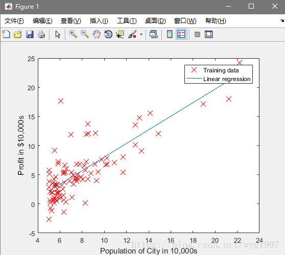
最后运行一下ex1.m验证代码:
扫描二维码关注公众号,回复:
1651772 查看本文章
